


CellTool User Guide
2
TABLE OF CONTENTS
Introduction ................................................................................................................................................................... 4
Supported image file types ........................................................................................................................................ 4
Output files ................................................................................................................................................................ 4
License agreement ..................................................................................................................................................... 5
System requirements ..................................................................................................................................................... 5
Installation instructions.................................................................................................................................................. 6
Updates .......................................................................................................................................................................... 7
Profile settings ............................................................................................................................................................... 7
Top Menu ....................................................................................................................................................................... 7
File Menu ................................................................................................................................................................... 7
Edit menu ................................................................................................................................................................... 8
Help Menu ................................................................................................................................................................. 8
Data sources panel ....................................................................................................................................................... 10
Work Screen ................................................................................................................................................................. 12
ROI Manager ................................................................................................................................................................ 13
Raw image settings ...................................................................................................................................................... 17
Brightness And Contrast .......................................................................................................................................... 17
Metadata ................................................................................................................................................................. 17
Processed image settings ............................................................................................................................................. 18
Histogram ................................................................................................................................................................ 18
Convolution ............................................................................................................................................................. 18
Segmentation........................................................................................................................................................... 20
Tracking Particles ..................................................................................................................................................... 21
Spot Detector ........................................................................................................................................................... 21
Results chart settings ................................................................................................................................................... 23
Auto Processing ............................................................................................................................................................ 24
Results Extractor PlugIn ............................................................................................................................................... 25
Results Extractor Solver ........................................................................................................................................... 27
Output file structure: ............................................................................................................................................... 29
Statistical equations used for the calculation of the results: .................................................................................. 30
Examples ...................................................................................................................................................................... 31
Measuring DNA-repair foci ...................................................................................................................................... 31
Image analysis: ..................................................................................................................................................... 32
CellTool User Guide
3
Further processing of the acquired data in the Results Extractor Plugin. ............................................................ 35
FRAP Analysis ........................................................................................................................................................... 37
Image analysis: ..................................................................................................................................................... 37
Further processing of the FRAPA data in the Results Extractor: .......................................................................... 40
Developer guide ........................................................................................................................................................... 44
TifFileInfo class ........................................................................................................................................................ 45
ROI class ................................................................................................................................................................... 46
References: .................................................................................................................................................................. 47
CellTool User Guide
4
INTRODUCTION
CellTool is a stand-alone open source software with Graphical User Interface that
combines image analysis and real time data visualization. It has implemented algorithms for fast
automatic segmentation of big time-lapse image stacks. This software is designed to process noisy
images and is optimized for tracking objects such as cell nuclei and DNA repair foci over time. It
has a plugin engine and an integrated file browser for fast and easy access to the images. The
data obtained from the image analysis is dynamically displayed on a chart which allows the user
to observe the results simultaneously with the image processing. Custom functions can be applied
to the image processing which saves time and eliminates most of the post-processing steps of the
measured data. With the “Results Extractor” plugin in CellTool, the summarized results from the
analysis of the image series can be graphically presented and fitted to a custom or predefined
mathematical model. CellTool possesses intuitive graphical interface, implements multiple image
processing algorithms and is capable of simultaneous data processing and data visualization
greatly facilitating the efficiency of the image analysis. It is perfect for rapid and robust live cell
image data analysis providing an all-in-one solution to numerous demanding tasks. That and the
feature for simultaneous visualization of the results makes CellTool a very useful and user-friendly
software for microscopy imaging facilities. For more information, visit our web site:
https://dnarepair.bas.bg/software/CellTool/
SUPPORTED IMAGE FILE TYPES
CellTool uses Bio-Formats library to read image data. It can open most of the available
formats for microscopy images. CellTool supports 8-bit grayscale images and 16-bit grayscale
images (RGB images are split into 3 separate grayscale images). List with the supported by
Bio-Formats image file types is available at the following URL:
https://docs.openmicroscopy.org/bio-formats/5.8.2/supported-formats.html
OUTPUT FILES
CellTool uses 8-bit grayscale TIFF or 16-bit grayscale TIFF to store image data. The
parameters obtained during the image analysis and the regions of interests (ROIs) from the ROI
Manager are stored in the file metadata. The ROIs can be separately stored as “.RoiSet” file. The
data calculated from the ROIs can be exported as TAB-delimited text file (with the button
“measure” from the “ROI Manager”)
CellTool User Guide
5
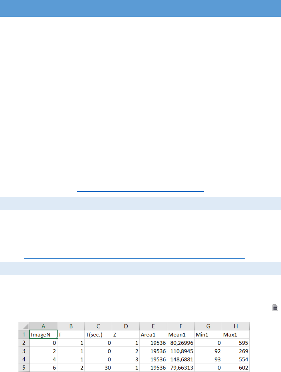
The first column is “ImageN” indicating the position of the current frame in the image
stack. For each frame column “T” shows the time slice index, “T (sec)” – the time in seconds and
“Z” – the position in the “Z stack”. Additionally 4 columns are added to the file for each ROI (ROI1,
ROI2,…,ROIn): “Area” (the size of the ROI in pixels), “Mean” (the average intensity value in the
ROI), “Max” (the maximal pixel intensity value) and “Min” (the minimal pixel intensity value).
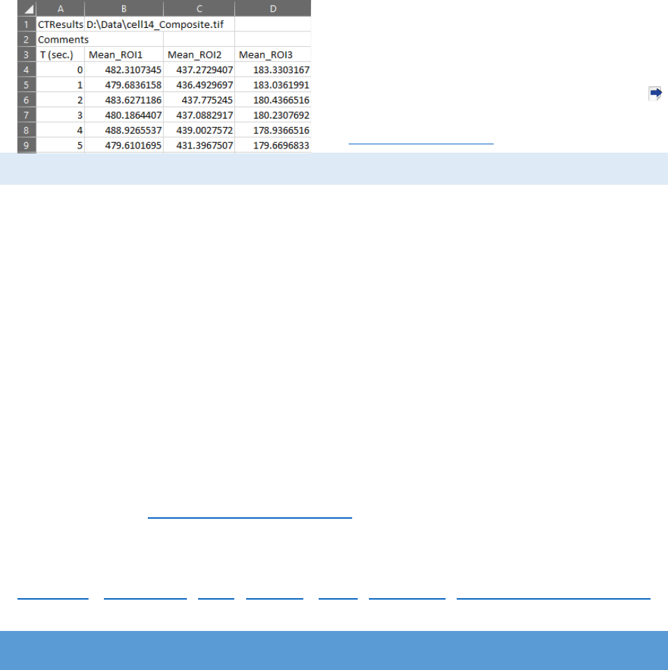
Important: CellTool has the ability to
export only a selected portion of this data in
separated TAB-delimited text file or even to
process the data with custom mathematical
functions and export the result (with the
“Export” button (Ctrl + E) in the tool strip menu).
See Results chart settings.
LICENSE AGREEMENT
CellTool - software for bio-image analysis
Copyright (C) 2018, Georgi Danovski
This program is a free software: you can redistribute it and/or modify it under the terms
of the GNU General Public License as published by the Free Software Foundation, either version
3 of the License, or (at your option) any later version.
This program is distributed in the hope that it will be useful, but WITHOUT ANY
WARRANTY; without even the implied warranty of MERCHANTABILITY or FITNESS FOR A
PARTICULAR PURPOSE. See the GNU General Public License for more details.
You should have received a copy of the GNU General Public License along with this
program. If not, see http://www.gnu.org/licenses/ .
This software is using the following libraries:
LibTiff.Net | Bio-Formats | ikvm | OpenTK | NCalc| Accord.Net| Microsoft Solver Foundation
SYSTEM REQUIREMENTS
Currently, CellTool can be installed on MS Windows 7 OS SP1 x64, MS Windows 8 OS
x64, MS Windows 8.1 OS x64, MS Windows 10 OS x64. It requires Microsoft .NET Framework 4.5
or higher to be installed.
CellTool can be installed on other operating systems with Windows Virtual Machine.
CellTool User Guide
6
INSTALLATION INSTRUCTIONS
1. Download and install “SetUp_CellTool.exe” from the following link:
https://dnarepair.bas.bg/software/CellTool/CellTool/SetUp_CellTool.exe
2. Run the “CellTool.exe” shortcut from the desktop.
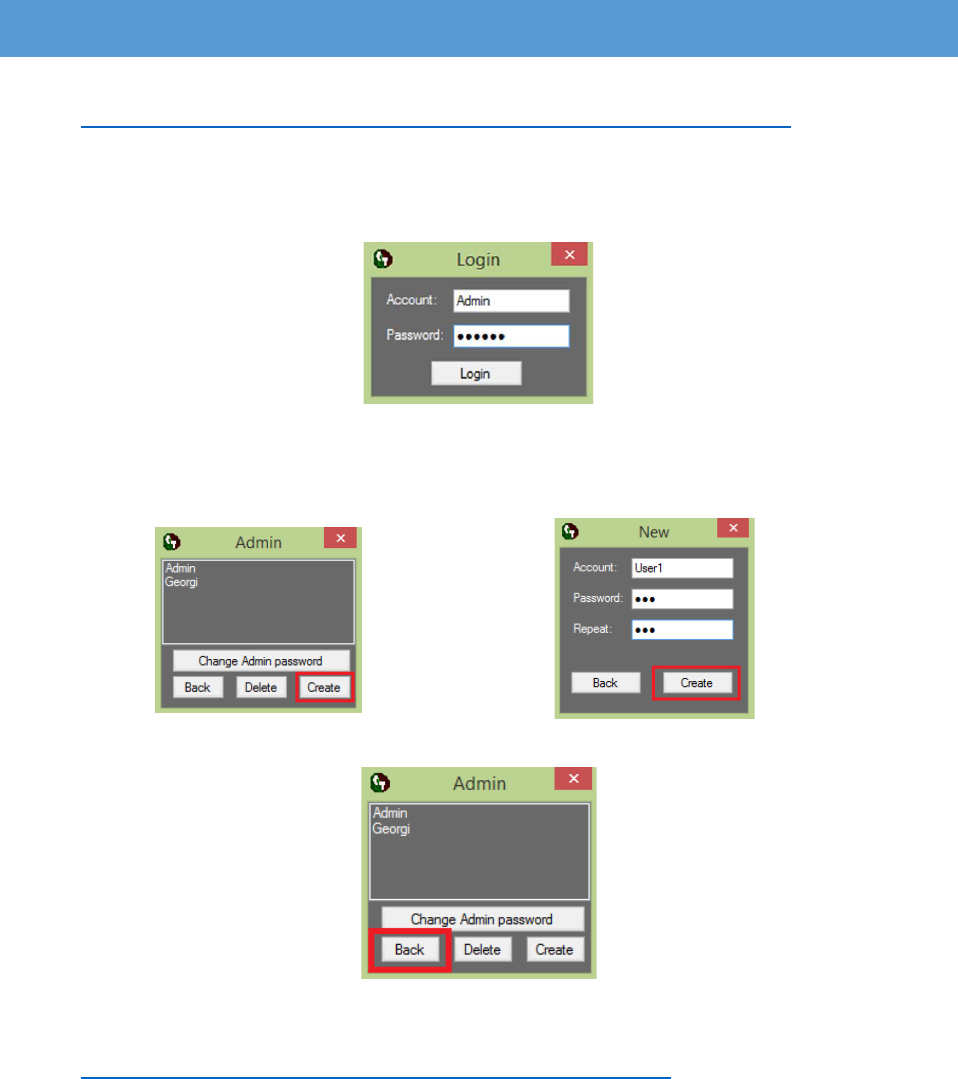
3. Login as "Admin" with password "123456".
(We recommend that you change the admin password immediately)
4. Create a new account by pressing the button “Create”. Change the admin password by
pressing the button “Change Admin password”. To delete the existing accounts select
them and press the button “Delete”.
5. Return to the login screen by pressing the button “Back”.
6. Login with the new account
7. Download a test image from the following link:
https://dnarepair.bas.bg/software/CellTool/Program/test.tif
CellTool User Guide
7
UPDATES
CellTool can be updated by accepting the update message when the software is started.
It is recommended to keep the software up to date.
PROFILE SETTINGS
The user profile is located in the upper right corner of the
program. For logging out and switching to another profile, “Log out”
must be pressed. The password can be changed with the “Change
password” option. Important: The account settings can be exported
with “Export settings” as .CTProfile and the file can be transferred to
another computer. The exported settings include the protocols for “Auto Processing”, “Hot Keys”
and “Smart Buttons” (see Help menu) that are created by the user. Exported settings can be
imported by pressing “Import settings” and browsing to the file.
TOP MENU
FILE MENU
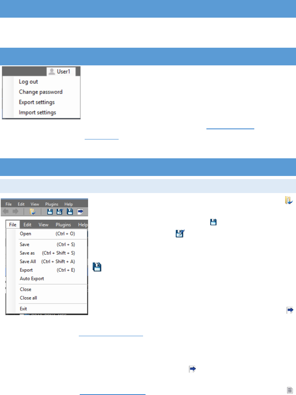
Images can be loaded to the program from the tool strip
“Open” button (Ctrl + O) or from the “File” menu. From there the
images can be saved or closed. The “Save” button saves the
current active image, the “Save As” button saves the active
image to a selected directory. Important: When attempting to
“Save As” an image, the default is the directory of the image. The
“Save all” button will save the changes made to all opened
images. From the “File” menu the buttons “Close” and “Close All”
will close the selected image or respectively all opened images. The
button “Exit” can be used for exiting the application. When closing
the program, it will exit without saving the unsaved images. The
“Export” button can be used for exporting the measured results for the checked ROIs and will be
discussed in the section “Results chart settings”.
With “Auto Export”, located in the “File” menu, the measured results will be automatically
exported in the image’s directory for all color channels. Two Results text files will be saved per
channel. First, the file that is usually extracted by pressing the “Export” button. It will carry the
name of the image and the color channel. It contains only the information from the settings
chosen by the user (see Results chart settings). Second, the file that is exported when the
CellTool User Guide
8
“measure” button in the ROI Manager is pressed, it will carry the name of the image, the color
channel and “_Results” at the end. It contains all the results, specified or not (see ROI Manager).
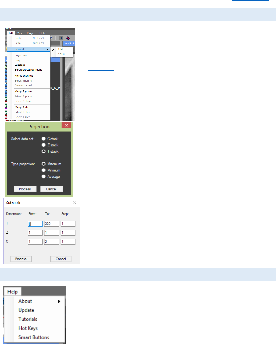
EDIT MENU
The “Edit” menu can be used to modify the image stack.
From “Convert”, the image type can be converted from 16 bit to 8
bit and from 8 bit to 16 bit. A selected ROI can be exported as a
new image in a new tab by pressing the “Crop” button (see ROI
Manager). Maximum Intensity, Minimum Intensity or Average
Intensity projection can be performed. If “Z stack” is selected it
will use the data from the Z stacks (all focal planes) for the
calculation and the result image will be with 1 Z plane. For T (time)
and C (color) stack projection the result image will be calculated
analogically from the T or the C stack.
Two image stacks can be combined into one with the
“merge” buttons. If “Merge Channels” is used the color channels
of the two images will be stacked together. ‘’Merge Z planes” will
add the Z planes of the second image to the Z planes of the first
image. ‘’Merge T slices” will add the T planes of the second image
to the T planes of the first image. With the “Extract channel/Z
plane/T slice” and “Delete channel/Z plane/T slice” buttons the
selected color channel, Z plane or T slice can be extracted to a new
tab or removed from the image. The “Substack” button in the
“Edit” menu can be used to create new image stack from the
source image by determining the first and the final Z, T or C frame
and the step for extraction (for example – every second T frame).
HELP MENU
Information about the license agreement of the software and the
list with the used libraries is available in the “Help” menu. The button
“Tutorials” opens new window with tutorials about the software.
CellTool allows to manually select keyboard shortcuts. This
option is available from the “Help”> “Hot Keys”. Every unassigned
keyboard button in combination with the “Ctrl” key can be used.
Shortcuts can be assigned to almost all tasks. Including the plugins and
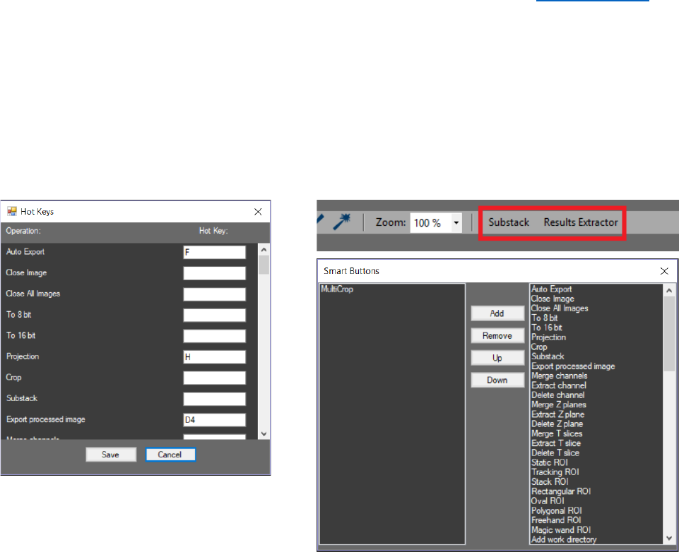
CellTool User Guide
9
already existing auto processing protocols (one hot key per protocol) (see Auto Processing).
Changes are applied when the “Save” button is pressed. If the key is already assigned a warning
message will appear. “Smart buttons” can also be assigned to a specific CellTool command, plugin
or auto processing protocol from the “Help”> “Smart Buttons”. By clicking on “Smart buttons” a
new window will appear, from there they can be added, removed or rearranged with “Up” and
“Down”. Once added the smart buttons will appear in the “Tool strip” menu after closing the
window “Smart Buttons”.
CellTool User Guide
10
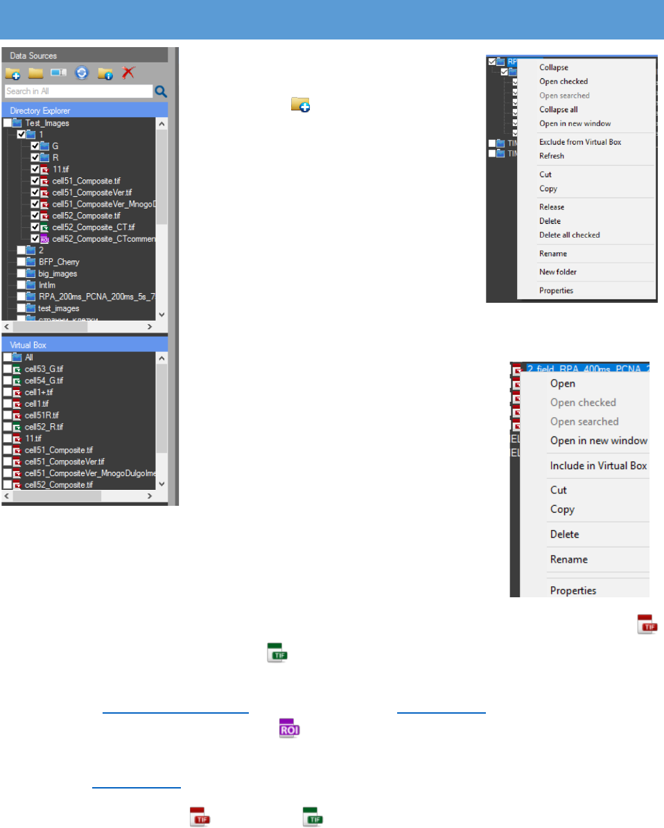
DATA SOURCES PANEL
The “Directory Explorer” panel
gives fast and easy access to the data. By
pressing the “Add work directory”
button a new directory can be added to
the tree view. With right mouse click on
an added work directory a context menu
appears. From there multiple options are
available. Important: An added work
directory can be removed from the tree
view with the “Release” button in the
context menu and it can be completely
deleted from its original directory with
the “Delete” option.
With right mouse click on an image
or a subfolder in the added directory a
slightly different context menu can be
activated (There is no “Release” option
there). With this controller, directories
and files can be opened, copied, cut or
pasted. They can be renamed or deleted. The properties of the image
can also be viewed. Important: The options in the context menu differ,
depending on if it’s an image or a subfolder that is selected and if there
are multiple images or subfolders checked.
There are three types of Icons visible in the “Directory Explorer”. The Red icon
indicates a raw image. The green icon indicates a processed image. The red icon turns green
if there is a text file with the same name as the raw image. This happens when the results from
the chart (see Results Chart Settings) or from the ROI (see ROI Manager) are saved with the same
name as the raw image. The purple icon indicates a ROI set created in the program. A ROI Set
file can be opened in the active image by double click or “drag and drop”. The RoiSet is channel
specific (see ROI Manager).
A single image (raw or processed ) can be opened with a double click on the name
or icon or “drag and drop” on the work screen from the “Directory Explorer” of CellTool. A single
CellTool User Guide
11
image can also be opened with “drag and drop” from the “File Explorer” of the computer to the
work screen
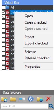
The “Virtual box” is the panel that allows for the extraction only
of images and RoiSets from the selected work directory and its
subdirectories. The images are automatically loaded to the virtual box
by checking the folder they’re in, from the directory explorer or by “drag
and drop”. The virtual box control has a context menu that can be
accessed with a right mouse click. It can be used for opening images and
releasing them from the virtual box. By pressing the “export” button the
images can be copied to a new directory on the hard drive. If “Export” is
clicked only the highlighted image can be exported to a new directory,
chosen by the user. If “Export checked” is clicked all checked images can
be exported.
There can be a search for a specific string. The search can be
performed in the “Directory Explorer” and/or the “Virtual Box”,
choosing between them can be done with a right mouse click in the
search box.
Groups of images can be opened with the “Open” buttons in the context menu. When
there are images in the tree view of the “Directory Explorer” or “Virtual Box” a context menu can
be activated with a right mouse click on a single image or a group of checked or searched images.
Then the images can be opened with “Open checked” or “Open searched”. “Open in new window”
can be used to open a folder from the tree view with the “File Explorer” on the computer.
Dragging a folder from the “Directory Explorer” of CellTool to the work screen will open all the
images in it.
CellTool User Guide
12
WORK SCREEN
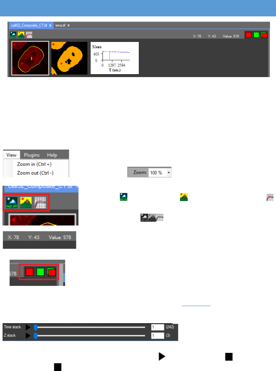
When the image is opened it is visualized in the central (work) panel. In the work panel
multiple images can be opened in different tabs. The tabs can be rearranged by dragging.
Additionally, an image can be closed by pressing the “X” button located next to the tab name.
In the work panel are the raw image, the processed image and the chart with the results.
These three images are available for every color channel. All the channels of the image are
displayed. The images can be resized by pressing the zoom in/zoom out buttons from the “View”
menu or with the hot keys “Ctrl + plus”/ “Ctrl + minus”. This can be
done with “Ctrl + mouse wheel up/down” or from the combo box
in the tool strip.
What is visualized on the work screen can be changed by
pressing the “Rаw Image”, the “Processed image” and the
“Results chart” buttons in the tab page menu. If these icons are grey,
they are not active ( ) and the image or chart are hidden.
When pointing the mouse cursor at a certain pixel the
coordinates and the value of the pixel are displayed at the end of
the tab page menu. The “Lookup Table” can be changed with a right
mouse click on the squares representing the color channels of the
image. The color channels can be disabled with a left mouse click.
They can be turned on at any time. Important: Even if one of the
channels is not visualized any region of interest (ROI) added to the
visible channel and then cropped (Edit menu) will be cropped from
the whole image not only from the visible channel.
At the bottom of the work
screen are two track bars. One
indicating the current position in the “Time stack” and the other the current position in the “Z
stack”. The clip will start by pressing on the play button , the icon changes to . By clicking on
the pause button the clip pauses.
CellTool User Guide
13
ROI MANAGER
The “ROI manager” is located in the “Properties” panel on the right edge.
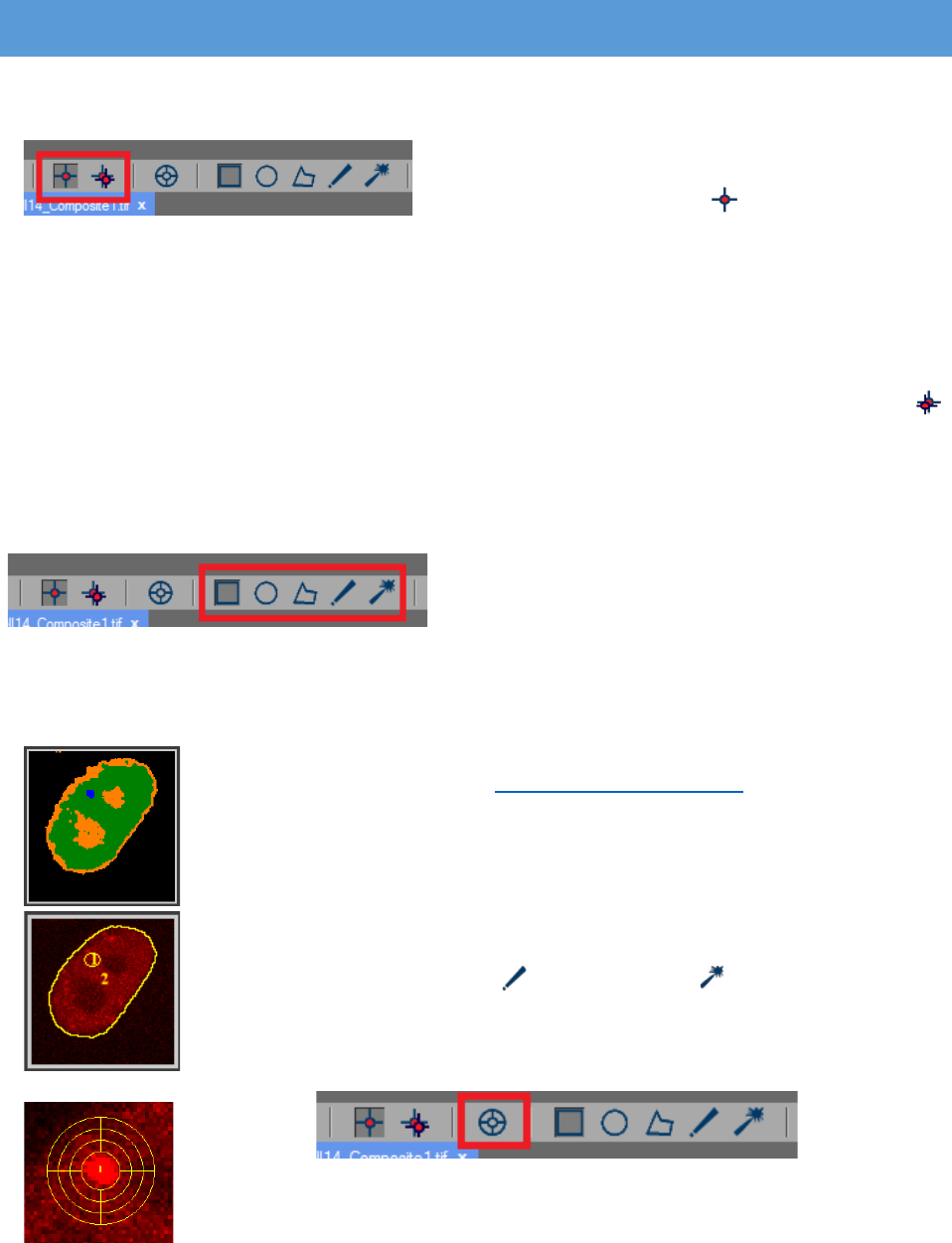
In the tool strip are two types of regions of
interest (ROIs) – static and tracking. The static ROI can
be enabled by pressing the “Static ROI” button.
The static ROIs are located at the same coordinates in
the time stack and the Z stack. They can be drawn only on the raw image. Every change made in
the static ROI is applied for the whole image. The coordinates of the “Static” ROI can be adjusted
for the whole image by dragging the ROI to another place or typing the desired coordinates in the
“Options” panel. The “Options” panel activates by clicking on the number of the ROI in the image
or on its name from the ROI manager. The tracking ROI can be enabled by pressing the
“Tracking ROI” button. It can be used for measuring moving objects. Multiple static and tracking
ROIs can be added. It is possible to switch between the two types of ROIs by clicking on the
corresponding ROI.
There are also different shapes for the ROIs:
Rectangle, Oval, Polygon, Freehand selection and
Magic wand. They can be found in the tool strip and
can be used for measuring the intensity of the pixels inside them. All the different shapes are
available for both type of ROIs.
The “Tracking ROI” can be used only on the “Processed image”. When
the image is segmented (see Processed Image Settings) every region in the
“Processed image” is with different color. A mouse click on the object of
interest ensures its tracking over time and will place a ROI that follows it. The
ROI however will be placed on the “Raw image”. The coordinates of the
“Tracking” ROI can be adjusted for a single frame by dragging the ROI in the
correct place or typing the desired coordinates in the “Options” panel. If the
shape of the ROI is “freehand” or “magic wand” it can be corrected on
a single frame by manually redrawing it with the “freehand ROI” on the “Raw
image” while pressing the keyboard button “Alt”.
There’s also the “Stack ROI” option in the tool strip. This function allows
for the creation of ROIs that are separated in layers. Each layer is measured
independently. It can be applied by combining it with the “Tracking ROI” or the
CellTool User Guide
14
“Static ROI”. The number of layers can be adjusted in the “Options” panel of the “ROI manager”
(“Stack:”), the width in pixels of the layers can be adjusted from “D:”. Infinite number of layers
can be added. The layered ROIs can be edited in the “Chart Series” panel when the “Results chart”
is activated (see “Results chart settings”). Every layer is divided in four subROIs: “Left Up”, “Right
Up”, “Left Down”, “Right Down”. Each of them can be included or excluded. Important: For the
ROI to be visible in the “Chart Series” it must be added first (Ctrl + T).
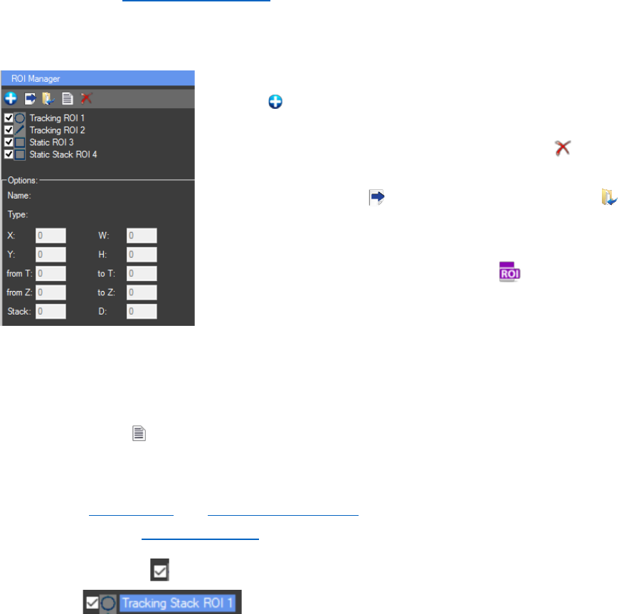
Once the ROI is created it can be added to the ROI list by
pressing “Add new ROI” button or “Ctrl + T”. A not yet added ROI
can be discarded with clicking the left mouse button somewhere in
the ROI manager. For deleting added ROI/s is the button (Ctrl +
D). Only selected (highlighted) ROIs can be deleted. In the “ROI
Manager”, buttons for exporting the ROI set files and loading
already existing ROI sets can be found. The ROIs are exported as
.RoiSet files that contain the information for the ROIs coordinates
in the image. Already existing ROI Set files can also be loaded to
the active image from the “Directory explorer” of CellTool with
double click or “drag and drop”. Important: The ROI set files are
channel specific. Even if the same ROI set is used for all color channels, the exported RoiSet file
will be for the channel of the image that was active at the time and if loaded will appear only on
that channel.
The button “measure” (Ctrl + M) exports a TAB-delimited text file for the selected color
channel with ALL the results from the ROIs, even those not specified by the user (For instance, in
the file for every ROI will be the X axis results for T slice, T(sec), Z slice and the same for all Y axis
options, see Output Files and Results Chart Settings). Important: This type of results file can’t be
used further in the “Results Extractor” plugin.
Only checked ROIs will be exported or measured. Important: Only selected ROIs can
be deleted . It doesn’t matter if they are checked or not. The ROIs are
selected with left mouse click on the name of the ROI from the “ROI Manager”, not on the
checkbox in front of the name. They can also be selected by clicking on the number of the ROI in
the “Raw image”. ROIs can be multi selected with holding “Ctrl” and left clicking on the desired
ROIs from the “ROI manager” or holding “Shift” and right clicking from the first desired ROI to the
last, if all ROIs need to be selected.
In the “Options” panel of the “ROI Manager” additional information about the selected
(highlighted, not checked) ROI can be found. From here the X and Y coordinates, width and height
for the Oval and Rectangular ROIs can be adjusted. The frame from which the ROI will be enabled
CellTool User Guide
15
in the time/Z stack can also be specified from here. Measurements will be performed only for the
selected intervals. For the “Stack ROI”, the number of layers (“Stack”) and the width in pixels for
the layers (“D”) can also be changed.
Important: The “ROI Manager” measures only the raw image. If
measuring of the intensity in the processed image is needed, it has to be
exported first. Pressing the “Export processed image” from the “Edit” menu
will open it in new tab.
The “Crop” option in the “Edit” menu can be used for cropping ROIs
out of the original image and exporting them as new images (for instance if there are multiple
cells on the image). For this option to work the ROIs must be added to the ROI Manager. Multiple
ROIs can be cropped at a time. Important: Only selected (highlighted) ROIs can be exported as
new images . It doesn’t matter if they are checked or not.
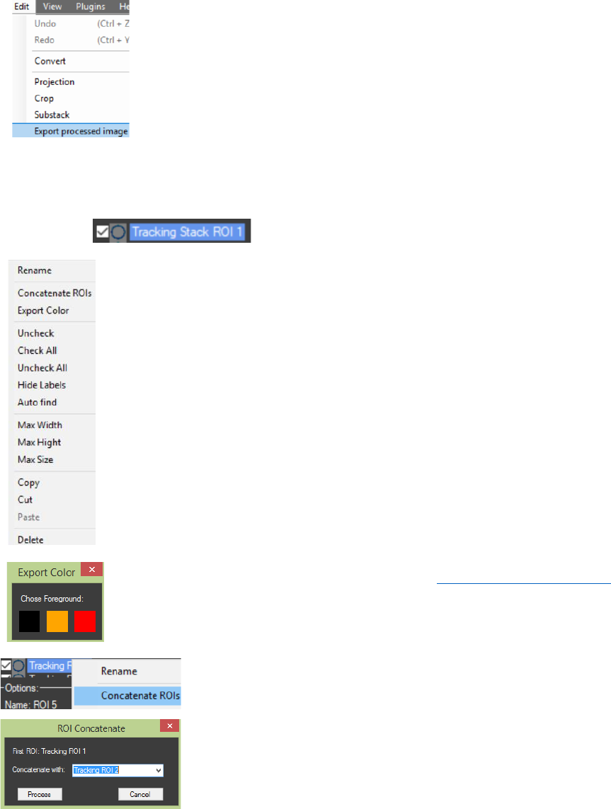
Context menus can be enabled: With right mouse click in the “ROI
Manager” a generalized context menu for all ROIs will appear. With right click on
a certain ROI in the “ROI Manager” a contexts menu containing specific options for
that ROI will appear. From the context menus the selected ROI/s can be Copied,
Cut and Pasted in other channel/image (ROIs can be copied and pasted between
the two channels in the image or in images in other tabs). The “Rename” option
can be used to add a comment/ label to the ROI. Also hot keys for “Copy” (Ctrl +
C), “Cut” (Ctrl + X), “Paste” (Ctrl + V) and selecting all ROIs (Ctrl + A) can be used.
Important: The order in which the ROIs are selected for “Copy” or “Cut” is the
order they are going to be Pasted in.
The button “Export Color” from the ROI Manager’s context menu can be
used to measure only the pixels with specific color (chosen by the user) in the
ROIs. The image must be segmented first (see Processed Image Settings). Results
will be automatically saved in the image directory. Every ROI is exported as a new
column.
“Concatenate ROIs” algorithm (ROI Manager Context menu)
can be used for merging several ROIs in one. Important: ROIs
(“static” or “tracking”) can be added only to a “tracking” ROI. Also
the time intervals must be properly adjusted before the
concatenation (example: for the first ROI “from T: 1 to T: 10” and for
the second ROI “from T: 11 to T: 300”). Only ROIs with the same
shape can be merged.
CellTool User Guide
16
In the ROI’s context menu there are options for “Max Width”, “Max Height”, “Max Size”
for a specific ROI. By choosing one of them, the program will automatically find and move the
cursor to the slice from the image stack where the ROI is with its max width, max height, max size
respectively.
“Static” ROIs can be added automatically to the ROI Manager by pressing the button “Auto
find” (ROI Manager Context menu). The program takes the coordinates of the ROIs (FRAPA or
microiradiation points) from the metadata of the image automatically if the images are acquired
with IQ3 software (ANDOR). To import the ROIs from other type of software the user has to create
a custom text file. The file must be named “RoiInfo.txt” and placed in the same folder as the
image. It must contain the following information:
<file name {with extension}>=<ROI shape {oval, rectangle, polygon, freehand}>(<coordinates>).
The coordinates for oval and rectangular ROIs are the upper left X, the upper left Y, the width and
the height values (Cell1.tif=oval(X, Y, Width, Height)). For polygonal and freehand ROIs the
coordinates include the X and the Y values of every angle in the proper order
(Cell2.tif=polygon(X1,Y1,X2,Y2,…,Xn,Yn)). ROI information can be stored in the same “RoiInfo.txt”
file for more than one image.
For example:
Cell1.tif=oval(200,200,20,20)
Cell1.tif=rectangle(200,200,20,20)
Cell2.tif=polygon(250,250,250,280,280,280,280,250)
Cell3.tif=freehand(250,250,250,280,280,280,280,250)
CellTool User Guide
17
RAW IMAGE SETTINGS
The raw image settings can be
accessed with left mouse click on the raw
image displayed in the work panel. The
content of the “Properties” panel on the
right will change and the “Brightness And
Contrast” settings, the “Metadata” and
the “ROI Manager” will become visible.
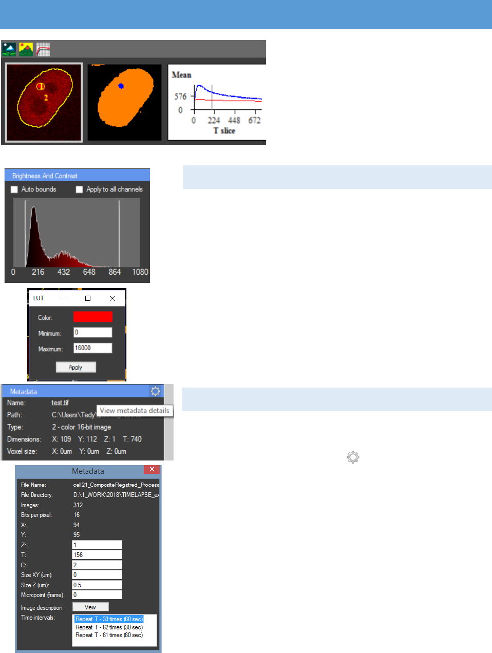
BRIGHTNESS AND CONTRAST
The brightness and contrast can be manually
adjusted by dragging the two vertical white lines. With a
right mouse click on the histogram a new pop up window
“LUT” will appear. Here the lookup table of the channel can
be changed. Also the settings can be adjusted by typing in
the new values.
If “Auto bounds” is checked the brightness and
contrast will be automatically adjusted for every frame. If
“Apply to all channels” is checked adjusted settings will be
applied to both channels.
METADATA
In the “Metadata” panel a short description of the
image is presented. The directory of the image can be seen,
its type and dimensions. If the “View metadata details”
button is pressed a new window will appear with basic
metadata of the image. Here the metadata can be edited. C,
T and Z values can be changed and the time intervals in the
image stack can be edited. Important: Sometimes, when the
metadata tags are not correct, the Time stack (T) and Z stack
(Z) values are switched. They can be adjusted here by typing
them in the correct manner to switch them back. Pressing
“View” next to “Image description” will open the full
metadata of the image.
CellTool User Guide
18
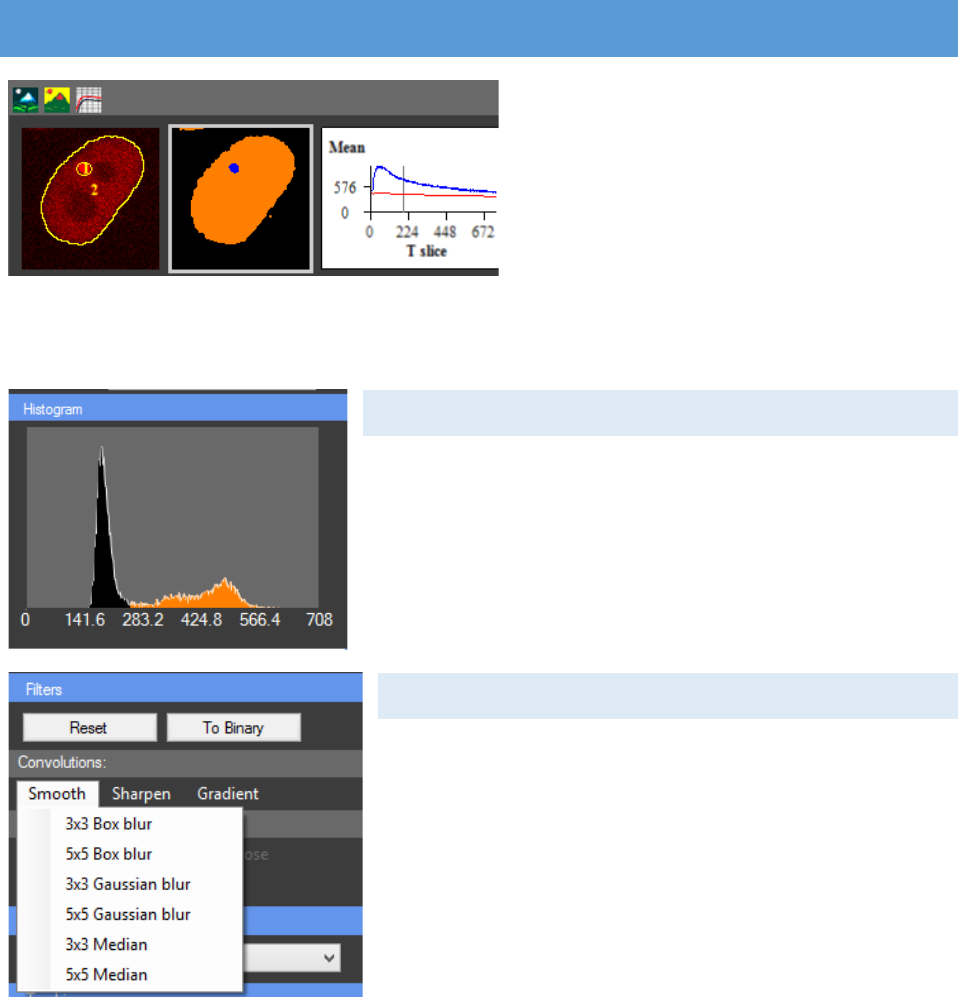
PROCESSED IMAGE SETTINGS
The processed image settings can
be accessed with a left mouse click on the
processed image displayed in the work
panel. The content of the “Properties”
panel will change and the image
processing settings – “Histogram”, filters
(“Convolution”), “Segmentation”, “Spot
Detector” and “Tracking” particles will
become visible.
HISTOGRAM
This histogram is showing the distribution of pixels,
based on their intensity, among the segmentation classes.
CONVOLUTION
Different image filters can be applied. They are
divided in two major categories: Convolutions and Binary
operations. The convolution filters multiply kernel matrix
to the image and return the result image. Three types of
convolutions are available – Smoothing, Sharpening and
Gradient detection. In the following table all available
kernel matrixes are shown.
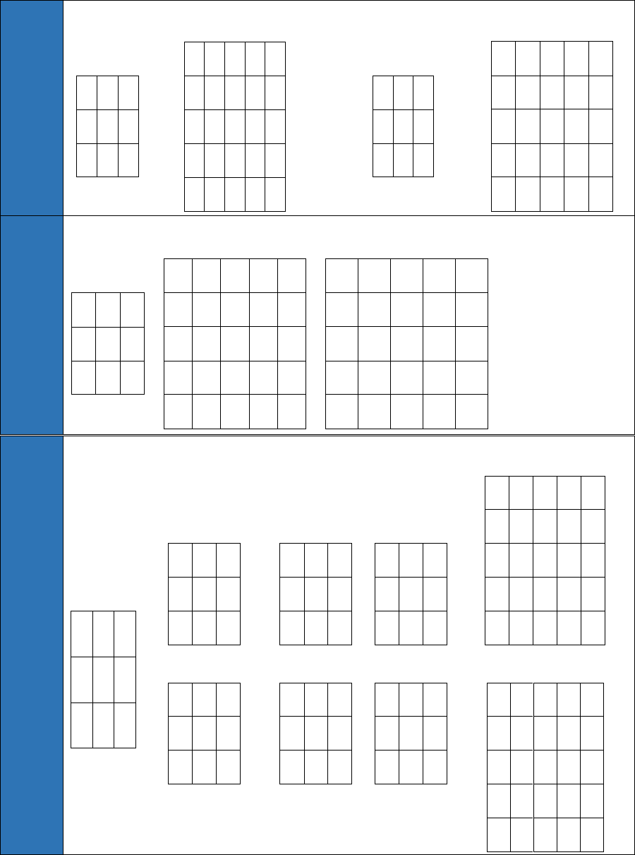
CellTool User Guide
19
Smooth
3x3 Box blur
1
1
1
1
1
1
1
1
1
5x5 Box blur
1
1
1
1
1
1
1
1
1
1
1
1
1
1
1
1
1
1
1
1
1
1
1
1
1
3x3 Gaussian blur
1
2
1
2
4
2
1
2
1
5x5 Gaussian blur
1
4
6
4
1
4
16
24
16
4
6
24
36
24
6
4
16
24
16
4
1
4
6
4
1
Sharpen
3x3 Sharpen
0
-1
0
-1
5
-1
0
-1
0
5x5 Sharpen
-1
-1
-1
-1
-1
-1
2
2
2
-1
-1
2
8
2
-1
-1
2
2
2
-1
-1
-1
-1
-1
-1
5x5 Unsharp masking
1
4
6
4
1
4
16
24
16
4
6
24
-476
24
6
4
16
24
16
4
1
4
6
4
1
Gradient
3x3
Edge
detection
-
1
-
1
-
1
-
1
8
-
1
-
1
-
1
-
1
3x3 Gradient detection
-1
-1
-1
0
0
0
1
1
1
-1
0
1
-1
0
1
-1
0
1
3x3 Sobel operator
-1
-2
-1
0
0
0
1
2
1
-1
0
1
-2
0
2
-1
0
1
3x3 Embos
-1
-1
0
-1
0
1
0
1
1
0
1
1
-1
0
1
-1
-1
0
5x5 Embos
-1
-1
-1
-1
0
-1
-1
-1
0
1
-1
-1
0
1
1
-1
0
1
1
1
0
1
1
1
1
0
-1
-1
-1
-1
1
0
-1
-1
-1
1
1
0
-1
-1
1
1
1
0
-1
1
1
1
1
0
CellTool User Guide
20
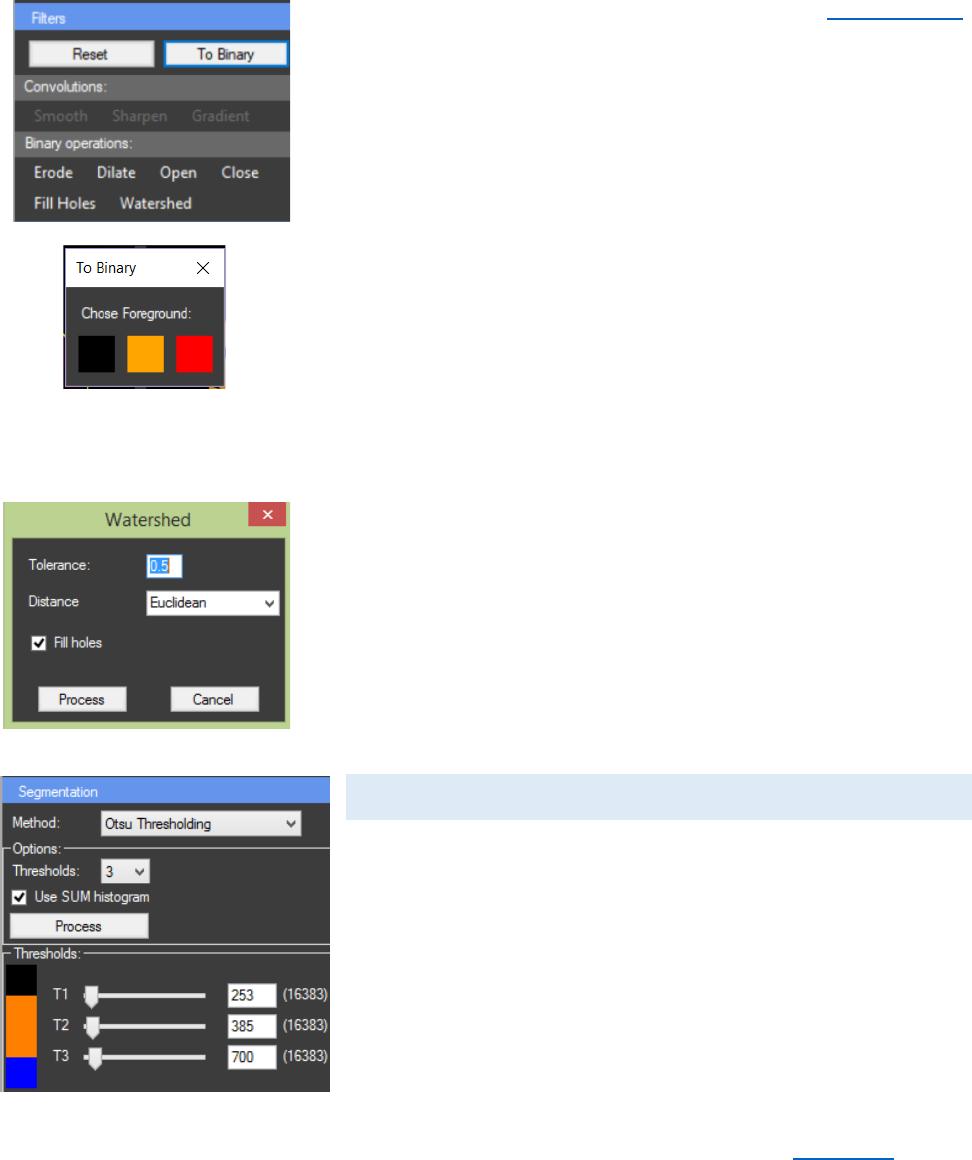
Binary operations can be applied after Segmentation
only if the image is converted to binary. By clicking the “To
Binary” button a new window will appear in which a foreground
color has to be chosen. Afterwards the panel “Binary
operations:” is activated from it different operations can be
applied. “Erode” can be used for removing one-pixel layer from
the foreground. “Dilate” can be used for adding one-pixel layer
from the foreground. “Open” performs an erosion operation,
followed by dilation. This smoothens the objects and removes
isolated pixels. “Close” performs a dilation operation, followed
by erosion. This smoothens the objects and fills in small holes.
“Fill Holes” can be used to remove unwanted pixels with the
intensity of the background from the object of interest. It can
be combined with “Open”.
“Watershed” can be used on binary images in order to
separate touching objects. Tolerance level can be changed to
eliminate oversegmentation and undersegmentation. First part
of the algorithm calculates distance map from the image. There
are four types of distance transformation – Manhattan,
Euclidean, Squared Euclidean and Chessboard. If “Fill holes” is
checked that algorithm will be applied to the image before the
“Watershed”.
SEGMENTATION
From the “Methods” combo box a method for
segmentation can be chosen. From the “Options” panel the
number of desired thresholds can be selected. The algorithm
will start when the “Process” button is pressed. If “Use SUM
histogram” is NOT checked only the histogram of the current
frame will be used for the calculations. Otherwise the histogram
for the whole image stack will be calculated and then used for
the segmentation. After the process of segmentation, the panel
“Thresholds” will become visible. From there the calculated
thresholds can be manually adjusted. The “Histogram” chart
can be used to view the distribution of the pixels between the
calculated thresholds.
CellTool User Guide
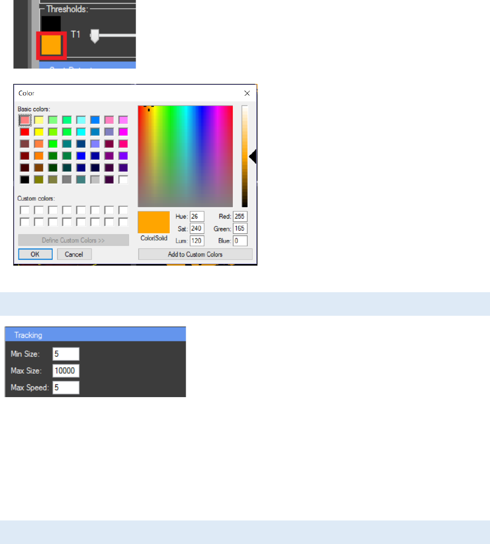
21
With a left mouse click on the colored button next to
the threshold this class of pixels can be disabled and they will
appear with their original color on the work screen. With a
right mouse click on this button the color of this group of
pixels can be changed.
Important: If the same color is
assigned to two or more classes of pixels
they will be recognized as one class from the
tracking algorithm.
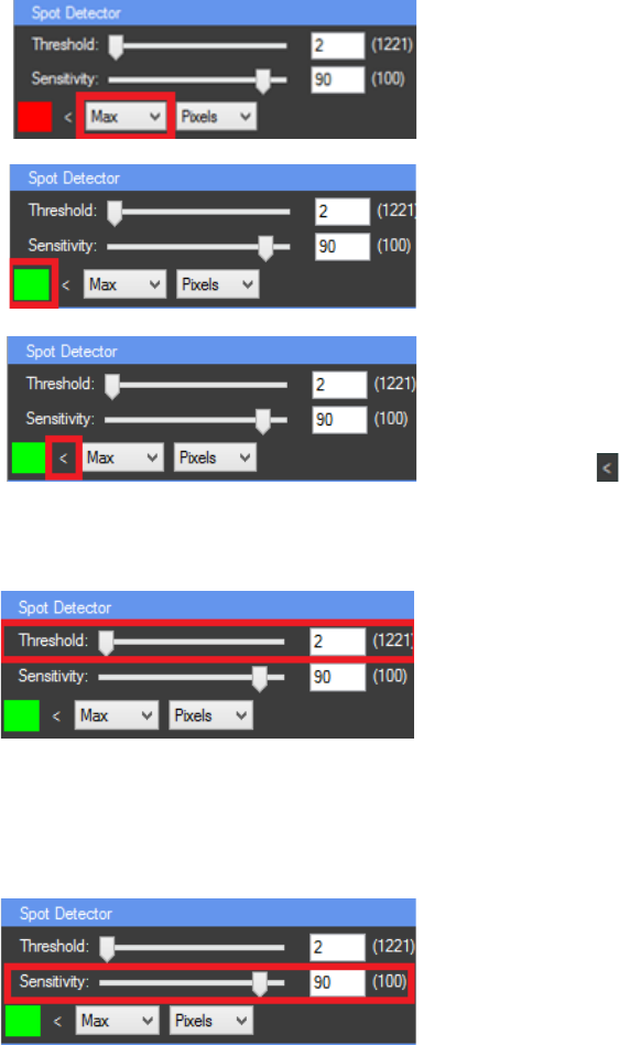
TRACKING PARTICLES
In the “Tracking” panel three parameters can be
adjusted. That can help improve the accuracy of the
tracking algorithm. “Min Size” is the minimum size in pixels
of the tracked object. “Max Size” is its maximum size in
pixels. If an object with the desired size is not found on
some of the slices in the image, the last calculated ROI will be used there. The algorithm is
calculating the center of mass for each T slice where the object appears. The object is added to
the tracking ROI only if the distance of translation in pixels is less than the “Max Speed”
parameter. If the object of interest is moving fast, the speed should be increased. The tracking
algorithm starts from the selected T slice and moves forward and backward to the end or
beginning respectively of the image stack.
SPOT DETECTOR
The “Spot Detector” panel can be activated by clicking on the processed image. The spot
detector can be used for detection of brighter or darker spots in the image. It analyses the
histogram of the image and calculates the zones of interest. Then with the other features of
CellTool the detected regions can be tracked and measured overtime or just traced and
measured, depending on the type of the image (single image or stack).
CellTool User Guide
22
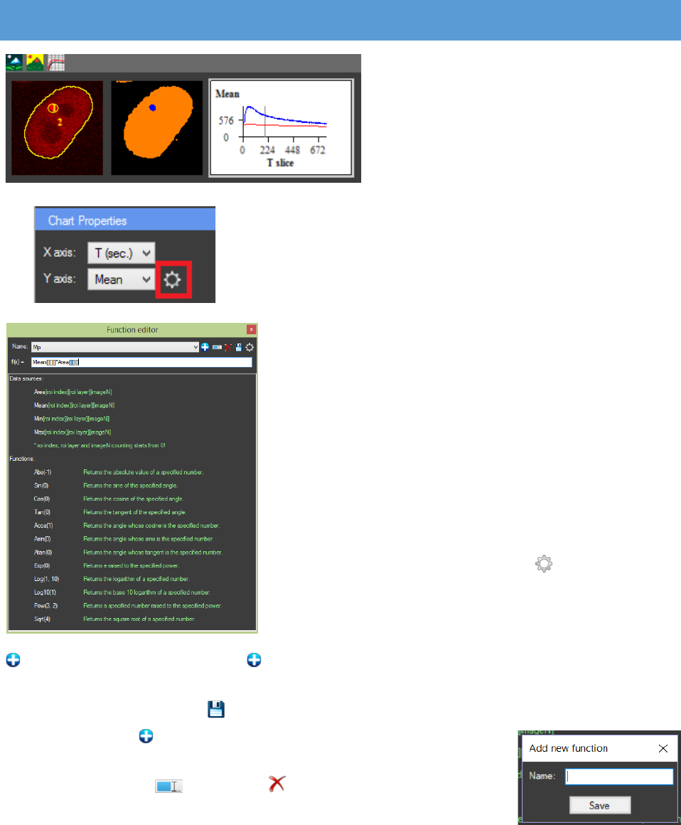
The first step in using the “Spot Detector” is to set
a “starting point” for the algorithm which can be Min (0
intensity), Max (the highest intensity value that occurs in
the image) or a threshold (T1 for the first threshold, T2 for
second…, T4 for fourth).
The color of the detected spots can be changed by
right mouse click on the “color button”.
The next step is to choose the zone of interest
with higher intensity (“>”) or with lower intensity (“<”)
then the selected starting point. Switching between
higher (“>”) or lower intensity (“<”) can be done by
clicking on the button.
The algorithm starts from the “starting point” and
counts the pixels. If the number of pixels is less than the
selected threshold value, the algorithm checks the next
intensity pixel group (with lower or higher intensity
depending on the selected option – “<” or “>”). This
process continues until it reaches an intensity pixel group
with number of pixels higher than the selected threshold
value. All checked pixels are included in the zone of
interest.
The histogram curve can be smoothed by
lowering the sensitivity value. This will reduce the
number of pixel intensity groups by merging the closest
groups into one depending on the selected sensitivity
value. This will affect the quality of the spot detection
process
CellTool User Guide
23
RESULTS CHART SETTINGS
The results chart settings can be
accessed by a left mouse click on the
results chart displayed in the work panel.
The content of the properties panel will
change and the chart settings will
become visible.
What is visualized on the axis can be changed. For
the “X axis” it can be chosen between T slice, T (sec.), Z
slice, T(min.) and T(hr.). To use T (sec.), T (min.) and T (hr.),
the time steps (if there are any) need to be set in the
metadata. For the “Y axis” it can be chosen between Area,
Mean, Min, Max, Total or a custom function. If “Area” is
chosen on the chart the size of the ROIs will be displayed.
“Mean” is average pixel intensity value, “Min” and “Max”
are respectively the minimal and maximal intensity value
of the pixels in the ROIs. “Total” represents the “Mean”
value multiplied by the “Area” of the ROI. Custom
functions can be applied by writing their formula in the
“Function editor”.
The function editor window can be accessed by
pressing the “Function editor” button next to the Y axis
combo box in the “Chart Properties” panel. The software
will calculate the selected function for each ROI and will
display it on the chart. The function editor can be used to
“Add new function”. When the is pressed a pop up window appears and in it the name of
the new function can be typed. Existing functions can be edited, after any changes are made they
can be saved by pressing the “Save function” (Important: if saving an edited function as a new
one is needed the “Add new function” button must be pressed, the
name can be changed and the function will be saved as a new one). The
functions can also be renamed or deleted. In the text box “f(x)”, a
custom function can be typed by using the CellTool format described in
the software.
Functions Mean, Max, Min and Area must be written with “[ROI index][ROI
layer][ImageN]” in the end. If the function has to be calculated for all ROIs and frames, empty
CellTool User Guide
24
brackets are needed: Mean[][][] * Area[][][]. If constant ROI index, ROI layer or frame is needed
it has to be specified. Example: If the first ROI needs to be subtracted from the mean value of
every ROI the following function is used: Mean[][][] – Mean[0][][]. This rule can be applied also
for the layer and the frame. The function can be checked for errors with the “Check for errors”
button. All functions available in the Ncalc library can be used.
The color of the chart series can be changed by a right mouse
click on its name in the “Chart Series” panel. Also the series can be
enabled or disabled by checking or unchecking them.
The “Export” button (Ctrl + E) can be used to save the data
visualized on the chart as a TAB delimited text file. By pressing it a safe
file dialog appears and in it the user can choose a specific name. The file
contains the information from the settings chosen by the user (for
instance for the X axis only Tsec. and for the X axis only Mean). This file
can later be used by the “Results Extractor” Plugin.
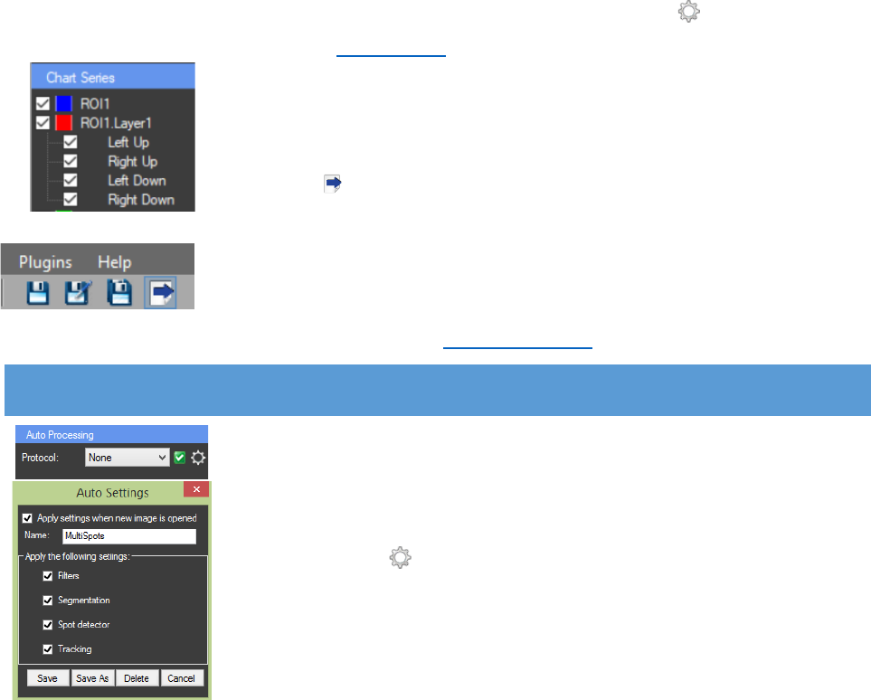
AUTO PROCESSING
At the top of the properties panel is a locked panel for “Auto
Processing”. It can be used for storing settings. After image processing
the steps of the process can be saved by creating a protocol. This can be
very helpful for fast processing of similar images. A protocol is created
by clicking on the next to “Protocol” in the “Auto Processing” panel.
Then a pop up window “Auto Settings” appears. There is a text box to
type the name of the protocol and an option to choose which settings
will be saved in the profile by checking or unchecking them. A
combination of filters and segmentation methods for instance. If the
“Apply settings when new image is opened” is checked, the settings will
be automatically applied to every newly opened image. The protocol is added by clicking “Save”.
After creating the first protocol, to create another one, the name of the protocol must be changed
and “Save As” must be clicked. If only the “Save” button is clicked the new protocol will be written
over the old one. Numerous profiles can be saved. A protocol can be deleted by pressing the
“Delete” button.
CellTool User Guide
25
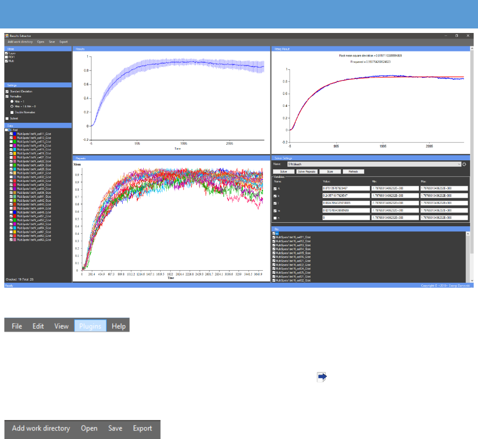
RESULTS EXTRACTOR PLUGIN
This plugin can be accessed from the button “Plugins” in the main menu
by choosing “Results Extractor”. It can be used for data processing of
the results from the image analysis. It uses as source data the text files acquired during the image
analysis with CellTool (the text files containing the exported information from the “Results chart”
in CellTool, the ones generated by pressing the “Export” button (Ctrl + E) in the main menu or
“Auto Export” from the “File” menu in CellTool.)
The results text files can be loaded to the “Result
Extractor” with the “Add work directory” button in the main
menu of the plugin. By pressing that button a directory browser appears and from it the user can
browse to the folder with the processed images and their text files. Important: If the last
processed image is still open in CellTool, the default folder in the directory browser is that of the
processed image. By clicking “OK” the information of all the processed images in this folder will
be loaded in the plugin automatically. The data from these files will be displayed on the “Repeats”
chart. There can be multiple folders from different directories added with the “Add work
directory” button. This can be helpful for combining data from experiments from different days
for instance. Once loaded to the plugin the data can be saved with “Save” as a text file with
“.CTData” extension. All the settings and changes will be stored and can be viewed later in the
plugin. The saved “.CTData” files can be reloaded by pressing the “Open” button. The results from
the plugin can be exported with “Export” as a TAB-delimited output text file and used in another
CellTool User Guide
26
software if needed. The information for the calculated fits, if there is any, and the formulas used
for fitting are also exported with everything else in the TAB-delimited text file.
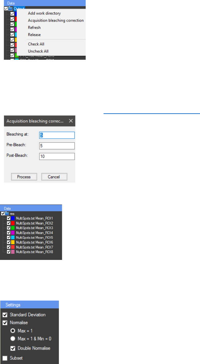
With a left mouse click in the “Data” panel a context menu
appears. Files can also be loaded to the plugin by pressing the “Add
work directory” button from there and browsing to the directory
where the files are located. The “Refresh” button reloads the text
files in the plugin. It can be used for loading text files from images
from the same data set processed after the plugin is opened. The “Release” button realeses
folders from the plugin. There is also the “Acquisition bleaching correction” option for
normalizing FRAPA data by applying two formulas, one for Double Normalization and one for
Full Scale Normalization [2] (See Further processing of FRAP data). Three parameters need to be
predefined in the “Acquisition bleaching correction” window. In
“Bleaching at:”, the number of the frame of the bleaching. In “Pre-
Bleach:” the amount of frames before bleaching. There must be at least
one frame before the bleaching. In “Post-Bleach:” the amount of
frames after bleaching.
The plugin will calculate automatically the average curve and the
standard deviation. They will be displayed on the “Results” chart. A certain
sample curve from the “Repeats” chart can be eliminated from the
average curve(“Results” chart) by unchecking its data series in the “Data”
panel. A certain curve can be highlighted (Bolded) by clicking on it in the
“Repeats” chart or selecting its name in the “Data” panel. The Y values of
both charts can be “Area”, “Mean”, “Min”, “Max”, “Total” or a custom
function, depending on the chosen option during the image processing
stage. Important: Theese parametars can’t be changed in the “Results
Extractor” once they are saved in the main program.
The normalised results can be viewed by checking the checkbox
“Normalise” in the “Settings” panel. If “Max = 1” is checked, the values
will be calculated by dividing the Y value of each data point by the maximal
Y value of the sample. If “Max=1 & Min=0” is checked, additionally the
minimal Y value of the sample (on the “Repeats” chart) will be subtracted
from each data point of the Y value, followed by dividing the maximal Y
CellTool User Guide
27
value. If activated, the “Double Normalise” option will recalculate the
average curve (on the “Results” chart) in order to normalise it by dividing
the Y value of each data point by the maximum Y value.
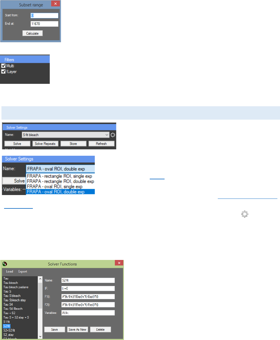
A subset can be created from the data set depending on the X values
(T slice, T(sec.), Z slice, T (min.) or T(hr.)) by using the “Subset” option.
When the checkbox next to “Subset” is checked, a popup window “Subset
range” appears. In this window the data set can be shortened. The original
data set can be restored by unchecking the checkbox.
Filters can be used to sort the “Data” tree view. They can be added
with a right mouse click in the “Filters” panel. Only the series that contain
the text written in the filter (in the name or in the comment) will be active.
Series that contain a specific text can be eliminated by adding “!” in the
beginning of the filter text.
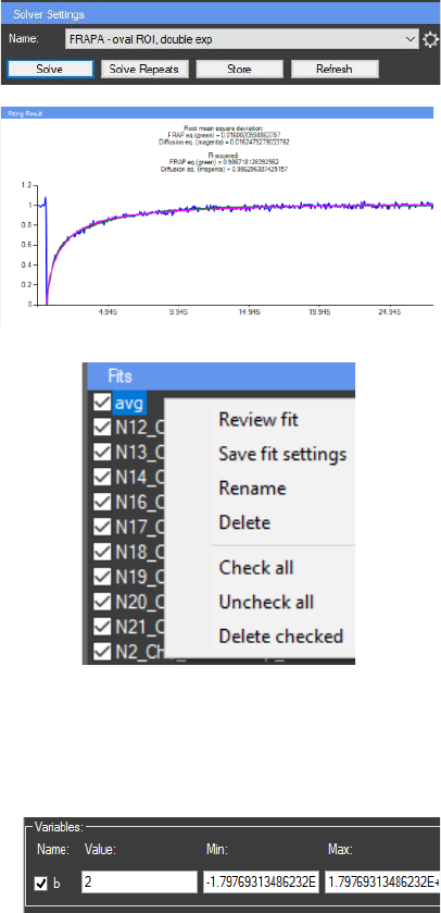
RESULTS EXTRACTOR SOLVER
The “Results extractor” can be used for fitting the
results to a predefined or custom mathematical model.
The predefined mathematical models are embedded in
the “Results Extractor”. There are four predefined
mathematical models for fluorescence recovery after
photobleaching (FRAP): “FRAPA-rectangle ROI, single exp”;
“FRAPA- rectangle ROI, double exp”; “FRAPA-oval ROI, single
exp”; “FRAPA-oval ROI, double exp” (see Further processing of
FRAP data). New models can be added to the program from the “Settings” panel, which is located
on the right, next to the “Results” and “Repeats” charts. By clicking on the button , a pop up
window “Solver Functions” will appear. The protocol is added by clicking “Save” or “Save As New”.
Unlimited number of constants and variables can be evaluated during the fitting process. Variable
“t” is reserved for the X axis values, and can’t be used, all other letters are free for defining new
variables. New variable is added by typing the name followed by “;”in the “Variables” text box. If
more than one variable is defined, all of them must
be separated with “;”.
Our solver supports the following arithmetic
operations: addition („+“), subtraction („-“),
multiplication („*“), division („/“), exponentiation
(„Pow[args]“,”Exp[val]”) and square root
(“Sqrt[val]”). “If statement” can also be used. The
CellTool User Guide
28
conditions of the “if statement” must be written in the “IF” text box. If the condition is fulfilled
the first equation “F1()” will be used for the calculations, otherwise the second equation “F2()”
will be used. If this statement is not required, in the “IF” text box only “t>=0” must be written.
Important: When the first custom mathematical model is ready it can be saved with the “Save”
button. For the next model to be saved, it has to be written over the old one and “Save As New”
must be pressed afterwards. If “Save As New” is pressed and the name of the new model is the
same as the old one both of them will be with the same name. If only “Save” is clicked it will
rewrite the new model over the old one.
Once created, the mathematical model can be
selected from the “Settings” panel. Important: Proper
initial values to the variables must be assigned in the
“Variables” panel. Pressing the button “Solve” will
start the solving algorithm. The current average curve
(from the “Results” chart) will be used аs source data.
When the fit data is calculated the result can be seen
in the “Fitting Result” chart. The result can be stored
in the “Fits” panel (located under the “Settings” panel)
by pressing the “Store” button. The button “Solve
repeats” activates the solving algorithm that uses the
current fit variables and solves the equation for all
samples in the “Repeats chart”. The fits for all the
repeats are automatically stored in the “Fits” panel
and can be viewed on the “Fitting result” chart one at
a time by double click. Multiple fits can be stored in
the “Fits” panel. The fits can also be reviewed with the
“Review fit” option in the “Fits” panel context menu.
The menu can be activated by right mouse click on a
fit in the “Fits” panel and can be used for renaming and
deleting stored fits. Also fit settings can be stored in an
existing fit by pressing “Save fit settings”.
The “Variables” panel provides access to the
values of the variables used to calculate the current fit
curve. The value of all variables can be manually
assigned in order to improve the performance of the solving algorithm. Also the range for
variation by the algorithm can be set (the defaults in “Min:” “Max:” are the minimal and the
maximal possible values). If the checkbox next to the variable name is unchecked this variable
becomes constant and will not be variated by the solving algorithm.
CellTool User Guide
29
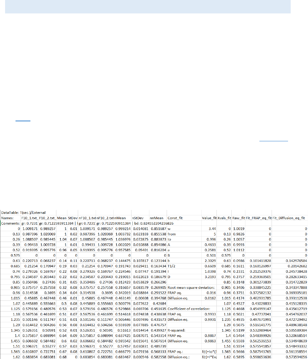
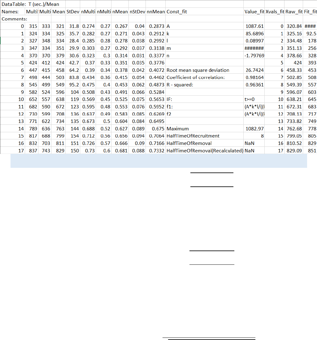
OUTPUT FILE STRUCTURE:
The results from the “Results Extractor” can be exported as TAB-delimited text file and will
contain: All samples, the average curve and the standard deviation. For the “Repeats” chart only
the results from the visible curves (filtered) and checked files in the “Data” panel will be calculated
and exported. Also samples (F10_1; F10_2), average curve (Mean), standard deviation (StDev),
normalized samples (nF10_1; nF10_2), normalized average curve (nMean), normalized standard
deviation (nnStDev) and double normalized average curve (nnMean) are included in the file.
For every calculated fit another 5 columns (or 6 for FRAP) are included: the variables names
(Const_[name of fit]), the variables values (Value_[name of fit]), the X axis data (Xvals_[name of
fit]), the Y axis raw data (Raw_[name of fit]), and the calculated Y axis fit data (Fit_[name of fit] or
if FRAP model is used there are two columns fit data - Fit_FRAP_eq_[name of fit] and
Fit_Diffusion_eq_[name of fit]). Below the constants additional statistical information about the
fit is available - root mean square deviation, coefficient of correlation, R – squared (the equations
are shown below). For FRAP, because two equations are used for the fitting, all these values are
calculated for both of them. If the set is not FRAP set, the maximum Y axis value, the half time of
recruitment, the half time of removal and the recalculated time of removal (if the fit curve never
reaches the 0 Y axis value) are also calculated. The formulas used in the mathematical model are
also shown. Example output file structure:
For FRAPA:
CellTool User Guide
30
All other Fits:
STATISTICAL EQUATIONS USED FOR THE CALCULATION OF THE RESULTS:
Standard deviation
Where:
is the sample mean;
is the individual sample point indexed with ;
is the sample size;
Root mean square deviation
Where:
are the predicted values;
is the individual sample point indexed with ;
is the number of observations;
Correlation coefficient
Where:
is the sample size;
and
are the individual sample points
CellTool User Guide
31
indexed with ;
and are the sample means;
is the number of observations;
R - squared
Where:
is the sample size;
and
are the individual sample points
indexed with ;
and are the sample means;
is the number of observations;
EXAMPLES
MEASURING DNA-REPAIR FOCI
The DNA of every cell is under a constant attack by various mutagenic factors which
damage the DNA and can cause cell cycle arrest and even cell death. Accumulation of DNA
damage is the basis for cancer development and one of the reasons for aging of the organisms.
In order to preserve the integrity of their DNA, cells have evolved an impressive array of DNA
repair pathways, which are precisely coordinated with the progression of the cell cycle. Recently
published article demonstrates a method for characterization and evaluation of the process of
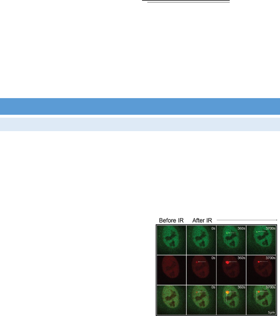
DNA repair by using time-laps fluorescence microscopy of living cells [1]. The model object for
these studies is the "HeLa Kyoto" cell line. The cells are transfected with the genes for the proteins
of interest fused with a fluorescent protein (EGFP or
mCherry). Ultraviolet laser is used to induce lesions
in DNA by irradiation (IR) of a small part of the cell
nucleus. The expression levels and localization of
these proteins are detected due to the fluorescent
protein component by measuring the intensity of
the pixels in the area of damage. The proteins
involved in the process of DNA repair can be
characterized by measuring the kinetics of
recruitment and removal at the sides of DNA lesions.

CellTool User Guide
32
Here we propose the following protocol for semi-automatic analysis of DNA-repair foci.
Properties of the test images: 16-bit grayscale TIF; 3 focal planes with 0.5 um between
each; Time interval between 1s and 5s depending on the recruitment time of the examined
protein. The images are of living HeLa Kyoto cells acquired with a spinning disk confocal
microscope with a UV laser module and recorded with the IQ3 software of Andor. Detailed
information for the test images like laser exposure, UV laser intensity, ext. can be found in the
image metadata (see Metadata).
Test data sets:
Test data set can be downloaded as an archive from the following URL:
https://dnarepair.bas.bg/software/CellTool/DataSet/MP_DataSet.rar
The MP_DataSet archive contains the following test data:
1. RawDataSet_RNF168 folder – with the raw images from the microscope;
2. CroppedDataSet_RNF168 folder – with cropped single cell images with Maximum
intensity projection;
3. ProcessedDataSet_RNF168 folder - with the processed images and results text files;
4. Results_RNF168.CTData – the input file for the “Results Extractor” with NO
calculated fits;
5. Fit_Results_RNF168.CTData – the input file for the “Results Extractor” with
calculated fits;
6. Fit_Results_RNF168.txt - exported text file from the “Result Extractor” containing
all the measurements and fits;
IMAGE ANALYSIS:
1. Download the test data archive MP_DataSet and extract it to the hard drive.
2. Load the image stack (2_RNF168.tif):
a. From the “Data sources” panel press “Add work directory” icon and browse to the
RawDataSet_RNF168 folder with the sample images on the computer. Select “OK”.
The chosen folder will now be visible in the “Directory Explorer” of CellTool. Double
clicking on the folder will expand it and the images in it will be visible. Double clicking
on the 2_RNF168.tif image will open it in the work screen.
b. The image can also be opened by dragging it from the “File Explorer” of the computer
to the work screen.
CellTool User Guide
33
3. The raw images are in 3 focal planes (Z stack). Maximum intensity projection must be
performed for minimizing the effect of eventual vertical movement of the DNA-repair
foci.
- From the Top Menu press “Edit”> “Projection”. Select “Z stack” for data set, and
“Maximum” for type of projection.
4. Crop step: There are multiple cells in the original image, the processing can be performed
directly on it or the cells can be cropped from the original image, saved as different
images and then processed (use an image/s from the CroppedDataSet_RNF168 folder if
you want to skip this step)
- From the Tool strip menu select “Static ROI” and “Rectangular ROI” to draw the ROI.
- All of the cell nuclei that need to be measured have to be added to the “ROI
Manager” and selected (see ROI Manager).
- From the top menu choose “Edit”> “Crop”. All of the selected ROIs will be exported as
new images in new tabs.
- Save every cell as a different image “File”> “Save” or “Save as” if you want to change
the image name (we recommend “Save as” if you are working in the original image,
always keep the original image intact).
- Choose one of the cells for further processing.
5. Image filters need to be applied in order to minimize the effect of the noise over the
further image processing.
- Press the icon for the “Processed image” from the tab page menu to make it
visible and select the processed image to enable the options in the “Properties”
panel.
- We recommend Gaussian blur 5x5. In the “Properties” panel in “Filters”>
“Convolutions” select “Smooth”> “Gaussian blur 5x5”.
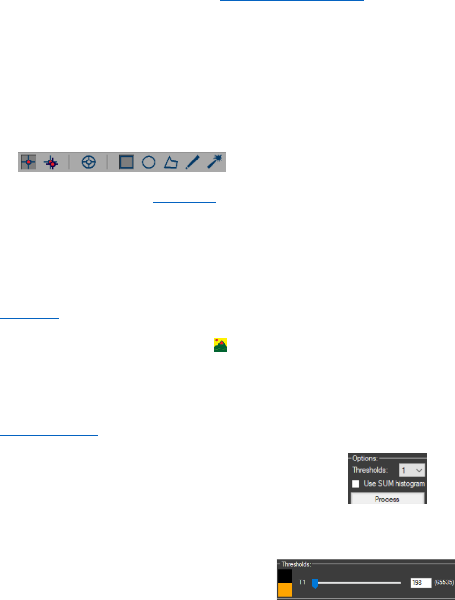
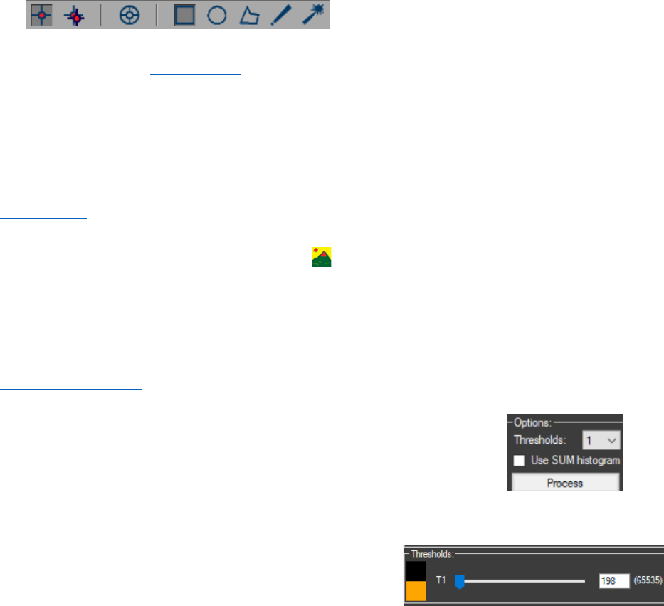
6. Image segmentation is performed by using K-means or Otsu thresholding with one
threshold. As a result, the cell nuclei must be successfully segmented.
- In the “Segmentation” panel for “Method” choose “Otsu
thresholding” or “K-means”, then an “Options:” panel will be
enabled in it set the number of “Thresholds” to 1.
- “Use SUM histogram” must be unchecked, for the segmentation only the current
frame will be used. The image should be on the first frame, because there is no DNA
repair focus there.
- Press “Process” to start the segmentation. If the
segmentation is not satisfying the threshold in the
“Thresholds” panel can be manually adjusted.
CellTool User Guide
34
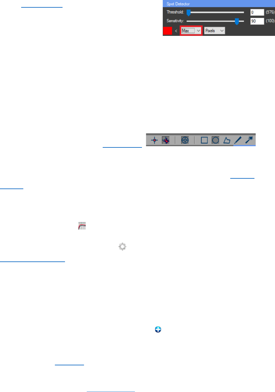
7. From the “Spot Detector”, the “Threshold” and
“Sensitivity” can be modified for better detection. Move
the track bar of the image forward a few frames (10-20)
to a point where the DNA repair focus in the cell
nucleus is visible to make sure it’s segmented.
- The combo box under “Sensitivity” must be set to “Max”. The highest intensity value
that occurs in the image. This is the starting point for the algorithm.
- The “Threshold” can be 0 for this set of images. It depends on the intensity of the
signal.
- The “Sensitivity” must be set to 90 for smoothing of the histogram and better results.
8. Tracking step: The automatic algorithm will track the DNA-repair focus throughout the
image stack.
- From the Tool strip menu select “Tracking ROI” and “Oval ROI”, enable the “Stack
ROI” option to draw the ROIs (see ROI Manager).
- With right mouse click in the segmented image (make sure it’s active) select the DNA-
repair focus (it will be colored in red).
- See if the algorithm tracked the DNA-repair focus correctly. If not, adjust the tracking
settings.
- Add the ROI to the ROI manager (Ctrl + T).
9. Results calculation: Here we are using a predefined formula to eliminate some of the
postprocessing steps:
- Enable the “Results chart” from the tab page menu to view the result.
- Select the chart to enable the “Chart Properties” panel.
- Open the “Function editor” by pressing from the “Chart Properties” panel (see
Results Chart Settings).
- In the f(x) text box add the following formula:
((Mean[][0][]-Mean[][1][])-(Mean[][0][N]-Mean[][1][N]))*Area[][0][]
(The N must be replaced with 5. N is the numeric value indicating the frame of laser
microiradiation. For the test data the microiradiation is at the end of frame 5. That is
why the bleach effect is visible on frame 6.)
- Give the function the name “Micropoint” and press “Add new function”.
- Select it from the Y axis combo box in the “Chart Properties” panel.
- Select T(sec) from the X axis combo box. If the time interval is not correct, it can be
changed from the metadata.
Important: After this step, the settings can be stored as new protocol and can be applied to
the other images automatically (see Auto Processing).

CellTool User Guide
35
10. Export all the results as Text files by pressing “File”> “Auto Export” (see File Menu).
11. Save the image with the changes. “File”> “Save” or “Save as”.
Important Note: Saving the image in CellTool will keep all the settings for that image like
ROIs, Segmentation, Results chart properties, everything. And the user can always return
later to view the image or extract more results if needed. There are preprocessed images in
the ProcessedDataSet_RNF168 folder.
FURTHER PROCESSING OF THE ACQUIRED DATA IN THE RESULTS EXTRACTOR PLUGIN.
The Results Extractor Plugin can be used to extract the information from the results files and
to calculate the mean value of each repeat of the experiment (see Output file structure). The
raw data can be fitted to a mathematical model (see Solver). For the test data CRC modeling
of protein kinetics was used, as described in the Aleksandrov’s paper [1]. The formula can be
loaded automatically by opening the “Fit_Results_RNF168.CTData” file from the processed
data set or manually in the “Results_RNF168.CTData”. The structure of the model is as
follows:
IF: t>=0
F1(): (A*k*l*m)*((1/((l-k)*(m-k)*(n-k)))*Exp[-k*t]+(1/((k-l)*(m-l)*(n-l)))*Exp[-l*t]+(1/((k-
m)*(l-m)*(n-m)))*Exp[-m*t]+(1/((k-n)*(l-n)*(m-n)))*Exp[-n*t])
F2():0
Variables: A;k;l;m;n;
Processing of the results and fitting them to a custom mathematical model in the “Results
Extractor” plugin:
1. Open the “Results Extractor” plugin: “Plugins”> “Results Extractor”.
2. Load the results to the “Results Extractor”:
a. From the ProcessedDataSet, the files can be automatically loaded to the plugin:
- Press “Add work directory” and browse to the folder with the text files.
b. Test results files can also be used: Results_RNF168.CTData with the raw results or
Fit_Results_RNF168.CTData with a preloaded formula and calculated fits.
3. For the tutorial we are using the test results file: Results_RNF168.CTData with no
preloaded formula.
- Press “Open”, browse to the “.CTData” file and select it.
4. Remove unwanted charts from the “Data” panel by unchecking them. They will not be
included in the exported file.
5. From the “Settings” panel “Normalization” must be checked, “Max=1 & Mean=0” and
“Double Normalize” are optional.

CellTool User Guide
36
6. Check “Subset” in the “Settings” panel and in the pop up window for “Start from:” type
25 sec and for “End at:” 2000 sec. We are doing that because the micropoint irradiation
is on the 5
th
frame which is the 25
th
second and 2000sec because the length of the two
raw tiff files the cells are generated from is different and it need to be the same.
7. Fitting of the result (Optional):
- From the “Solver Settings” panel press the next to the fit name combo box to load
the formula:
Name: Fit1
IF: t>=0
F1(): (A*k*l*m)*((1/((l-k)*(m-k)*(n-k)))*Exp[-k*t]+(1/((k-l)*(m-l)*(n-l)))*Exp[-
l*t]+(1/((k-m)*(l-m)*(n-m)))*Exp[-m*t]+(1/((k-n)*(l-n)*(m-n)))*Exp[-n*t])
F2():0
Variables: A;k;l;m;n;
- Type random different values in the “Variables:” panel (exp. A:1, k:0.5, l:0.6, m:0.7,
n:0) and press “Solve”.
- The fit will appear on the “Fitting Result” chart.
- Press “Store” and the new fit will appear in the “Fits” panel.
- Press “Solve Repeats” to fit the individual repeats. It will use the current values to find
the closest ones for every individual repeat. They will automatically appear in the
“Fits” panel with the names of the repeats.
- With double click on the individual repeats from the “Fits” panel they can be viewed
one by one in the “Fitting Result” chart.
8. Saving the results:
- With the button “Save” the measures made on the Results_RNF168.CTData can be
saved as new file, that includes the fits and the formula used for them and all other
changes made from the user.
- With the “Export” button all the information in the CTData file will be exported as a
tab-delimited text file that includes the fits, Normalization, Standard deviation, ext.
9. There is also a previously generated text file containing that information:
Fit_Results_RNF168.txt (see Output File Structure).

CellTool User Guide
37
FRAP ANALYSIS
Fluorescence recovery after photobleaching (FRAP) is a method for determining the
kinetics of diffusion through tissues or cells. It is capable of quantifying the two dimensional
lateral diffusions of a molecule thin film containing fluorescently labeled probes, or to examine
single cells. This technique is very useful in biological studies of cell membrane diffusion and
protein binding. Here we propose а protocol for semi-automatic image analysis of FRAP of nuclear
proteins fused with fluorescent protein.
Properties of the test images: 16-bit grayscale TIF; 1 focal plane. The images are of living
HeLa Kyoto cells acquired with a spinning disk confocal microscope and recorded with the IQ3
software of Andor. Detailed information for the test images like laser exposure for instance can
be found in the image metadata (see Metadata).
Test data sets:
Test data set can be downloaded as an archive from the following URL:
https://dnarepair.bas.bg/software/CellTool/DataSet/FRAP_DataSet.rar
The FRAP_DataSet archive contains the following test data:
1. RawDataSet_FRAP folder – with one raw test image from the microscope;
2. CroppedDataSet_FRAP folder – with cropped single cell images;
3. ProcessedDataSet_FRAP folder - with the processed images and results text files;
4. Results_FRAP.CTData – the input file for the “Results Extractor” with NO calculated
fits;
5. Fit_Results_FRAP.CTData – the input file for the “Results Extractor” with calculated
fits;
6. Fit_Results_ FRAP.txt - exported text file from the “Result Extractor” containing all
the measurements and fits;
The RawDataSet_FRAP_All archive contains all the raw images used for creating the
CroppedDataSet can be downloaded from the following URL:
https://dnarepair.bas.bg/software/CellTool/DataSet/RawDataSet_FRAP_All.rar
IMAGE ANALYSIS:
1. Download the test data archive FRAP_DataSet and extract it to the hard drive.
2. Load the image stack (FRAP.tif):
CellTool User Guide
38
a. From the “Data sources” panel press “Add work directory” icon and browse to the
RawDataSet_FRAP folder with the sample image on the computer. Select “OK”. The
chosen folder will now be visible in the “Directory Explorer” of CellTool. Double
clicking on the folder will expand it and the image in it will be visible. Double clicking
on “FRAP.tif” image will open it in the work screen.
b. The image can also be opened by dragging it from the “File Explorer” of the computer
to the work screen.
3. Crop step: There is one cell in the original image that is bleached, the processing can be
performed directly on it or the cell can be cropped from the original image, saved as
different image and then processed (use an image/s from the CroppedDataSet_FRAP
folder if you want to skip this step. Load it the same way as the FRAP.tif).
- From the Tool strip menu select “Static ROI” and “Rectangular ROI” to draw the ROI.
- The cell nucleus that needs to be measured has to be added to the “ROI Manager”
and selected (see ROI Manager).
- From the top menu choose “Edit”> “Crop”. The selected ROI will be exported as a
new image in a new tab.
- Save the cell as a different image “File”> “Save” or “Save as” if you want to change
the image name (we recommend “Save as” if you are working in the original image,
always keep the original image intact).
4. Image filters need to be applied in order to minimize the effect of the noise over the
further image processing.
- Press the icon for the “Processed image” from the tab page menu to make it
visible and select the processed image to enable the options in the “Properties”
panel.
- We recommend Gaussian blur 5x5. In the Properties panel in “Filters”>
“Convolutions” select “Smooth”> “Gaussian blur 5x5”.
5. Image segmentation is performed by using K-means or Otsu thresholding with one
threshold. As a result, the cell nucleus must be successfully segmented.
- In the “Segmentation” panel for “Method” choose “Otsu
thresholding” or “K-means”, then an “Options:” panel will be
enabled in it set the number of “Thresholds” to 1.
- “Use SUM histogram” can be checked, for the segmentation all frames will be
calculated.
- Press “Process” to start the segmentation. If the
segmentation is not satisfying the threshold in the
“Thresholds” panel can be manually adjusted.
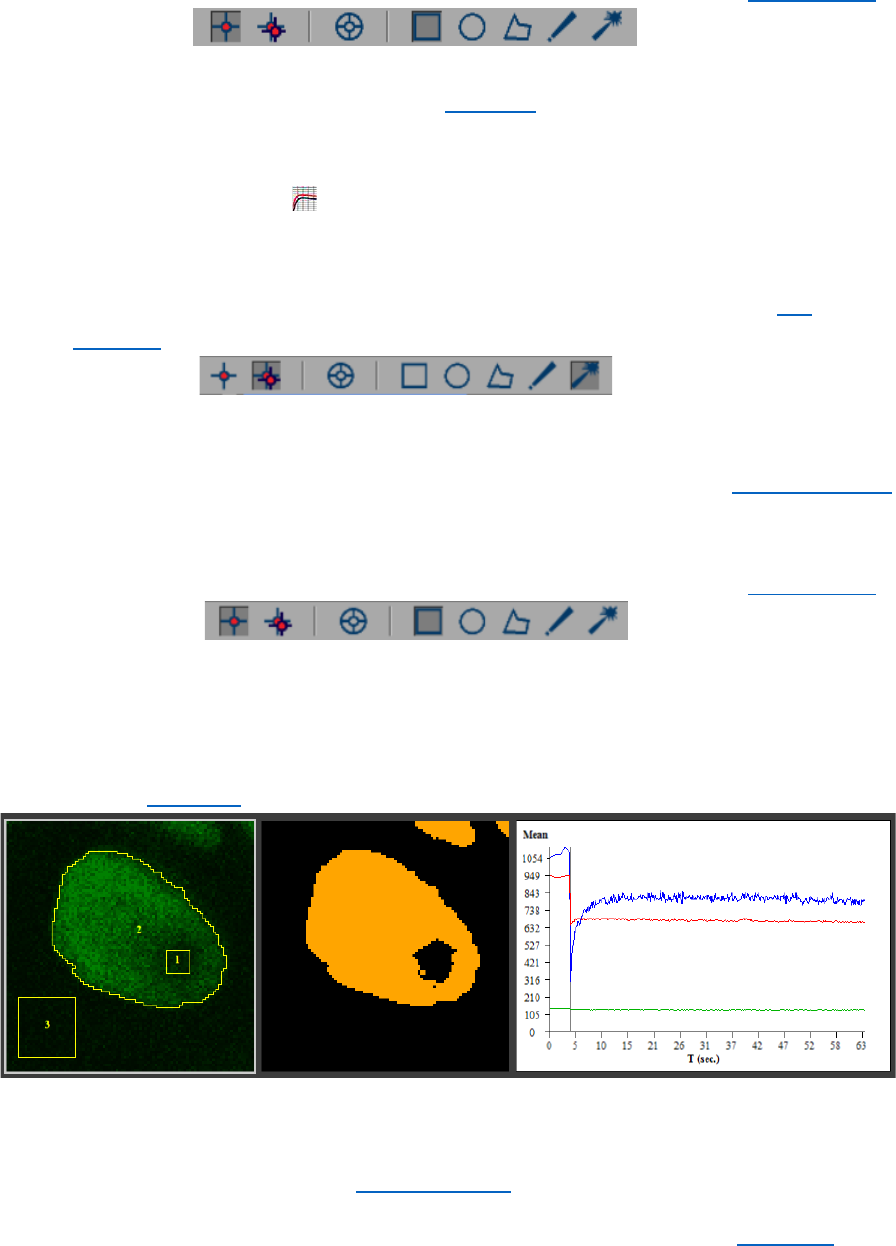
6. Measuring the intensity change at the region of photobleaching.
CellTool User Guide
39
- In the Tool strip menu select “Static ROI” and “Rectangular ROI” (see ROI Manager).
- Hold the right mouse button in the raw image (make sure it’s active) and draw a ROI
at the region of photobleaching. The “Auto find” option in the context menu of the
ROI manager can be used for convenience.
- Add the ROI to the ROI manager (Ctrl + T).
7. Enable the “Results chart” from the tab page menu to view the result.
8. Measuring the intensity of the whole cell nucleus. The automatic algorithm will track the
segmented nucleus throughout the image stack.
- In the Tool strip menu select “Tracking ROI” and “Magic wand ROI” (see ROI
Manager).
- With right mouse click in the segmented image (make sure it’s active) select the
nucleus (it will be colored in yellow).
- See if the algorithm tracked the nucleus correctly. If not, adjust the tracking settings.
- Add the ROI to the ROI manager (Ctrl + T).
9. Measuring the intensity of the background noise.
- In the Tool strip menu select “Static ROI” and “Rectangular ROI” (see ROI Manager).
- Draw the ROI somewhere in the background.
- Add the ROI to the ROI manager (Ctrl + T).
10. Select the Results chart to enable its “Properties”. Select “T(sec)” from the X axis combo
box and “Mean” from Y axis combo box. If the time interval is not correct, you can change
it from the metadata.
Important: after this step the settings can be stored as new protocol and can be applied to
the other images automatically (see auto processing).
11. Export all the results as Text files by pressing “File”> “Auto Export” (see File Menu).

CellTool User Guide
40
12. Save the image with the changes. “File”> “Save” or “Save as”. (We recommend not to
save over the original image files).
FURTHER PROCESSING OF THE FRAPA DATA IN THE RESULTS EXTRACTOR:
The Results Extractor PlugIn can be used to extract the information from the text files,
perform normalization, calculate the mean value of each repeat of the experiment and fit the
data to a FRAP model.
1. Open the “Results Extractor” plugin: “Plugins”> “Results Extractor”.
2. Load the results to the “Results Extractor”:
- A test results file can be used: Fit_Results_FRAP.CTData with calculated fits or
Results_FRAP.CTData with the raw results.
- Press the button “Open” in the Results extractor and browse to the
Results_FRAP.CTData file and select it.
3. In the “Settings” panel check “Subset” if only a portion of the result displayed on the
charts is needed. Nothing else needs to be specified.
4. Performing “Acquisition bleaching correction” in order to normalize the data by applying
two formulas, one for Double Normalization and one for Full Scale Normalization [2]:
Where:
– double normalized intensity;
– measured average intensity inside the bleached spot;
– measured average reference or whole studied compartment (cell, nucleus, etc.) intensity;
– measured average background intensity outside the cell;
Subscript _pre means the averaging of intensity in the corresponding ROI before bleach moment after
subtraction of background intensity;
Where:
- full scale normalized intensity;
- double normalized intensity;
- double normalized intensity at the time of the bleach;
- Right click in the “Data” panel of the Results Extractor to open a Context Menu
- In it choose “Acquisition bleaching correction”
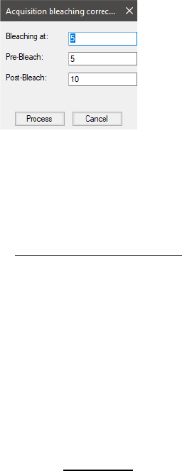
CellTool User Guide
41
5. Three parameters need to be predefined in the “Acquisition bleaching correction”
window:
- Next to “Bleaching at:”, the number of the frame of the bleaching must be specified.
In our case that frame is 5.
- Next to “Pre-Bleach:” the amount of frames before bleaching must be specified for
the pre bleach averaging. There must be at least one frame before the bleaching, any
number from 1 to 5 included will suffice in our case.
- Next to “Post-Bleach:” the amount of frames after bleaching must be specified for the
post bleach averaging.
Important: The gap ratio and the bleaching depth are automatically calculated and
stored as comment for each data series, they will be exported in the text file also. They are
calculated with the following formulas [3]:
Where:
– bleaching depth;
- averaging of the measured average intensity inside the bleached spot before
bleach moment after subtraction of background intensity;
– measured average intensity inside the bleached spot at the time of the
bleach after subtraction of background intensity;
Where:
– gap ratio;
- averaging of the reference or whole studied compartment (cell, nucleus, etc.)
intensity before bleach moment after subtraction of background intensity;

CellTool User Guide
42
- averaging of the reference or whole studied compartment (cell, nucleus, etc.)
intensity after bleach moment after subtraction of background intensity;
6. Remove unwanted curves from the “Data” panel by unchecking them. They will not be
included in the exported file.
7. Fitting of the result (Optional):
- Using the predefined models from the “Solver Setting” panel choose the name of the
proper model for the fitting.
- There are four predefined models: “FRAPA- rectangle ROI, single exp” ; “FRAPA-
rectangle ROI, double exp”; “FRAPA- oval ROI, single exp”; “FRAPA- oval ROI, double
exp”, that are combination of the following formulas:
One binding state model (single exp) [2, 4]:
Where:
– mobile fraction;
- unbinding rate constant [s
-1
];
– time after the bleaching [s];
Two binding states model (double exp) [2, 4]:
Where:
– mobile fraction;
- unbinding rate constants for the two binding states [s
-1
];
- fractions of bound molecules for the two binding states;
– time after the bleaching [s];
Diffusion model for rectangular ROI [2, 5]:
Where:
– normalizing coefficient to account the incomplete recovery;
- diffusion coefficient [µm
2
s
-1
];
- the width of bleach spot [µm];
– time after the bleaching [s];

CellTool User Guide
43
Diffusion model for oval ROI [2, 6]:
Where:
- modified Bessel functions.
– normalizing coefficient to account the incomplete recovery;
- diffusion coefficient [µm
2
s
-1
];
- the radius of bleach spot [µm];
– time after the bleaching [s];
8. In our case we are using the “FRAPA- rectangle ROI, double exp” model, because we
have two binding states and an oval ROI for the FRAPA region.
9. In the “Variables:” panel, for “w” fill the parameter in µm with the correct width for a
rectangular ROI or radius for an oval ROI.
- In our case in “w” we fill the width for a rectangular ROI, which is 2,3 µm.
- In “from” fill the bleaching frame number, in our case, that number is 5.
10. Press “Solve” and the calculated fit will appear on the “Fitting Result” chart.
11. Press “Store” and the new fit will appear in the “Fits” panel.
12. The model can be solved for each repeat individually if the button “Solve repeats” is
activated. They will automatically appear in the “Fits” panel with the names of the
repeats.
- Select them one by one from the “Fits” panel to view them on the “Fitting Result”
chart.
10. Saving the results:
- With the button “Save” the measures made in the Results_FRAP.CTData can be saved
as new file, that includes the fits and the formula used for them and all other changes
made from the user.
- With the “Export” button all the information from the CTData file will be exported as
a tab-delimited text file.
11. There is also a previously generated tab delimited text file containing that information:
Fit_Results_FRAP.txt (see Output File Structure).

CellTool User Guide
44
DEVELOPER GUIDE
Install your favorite IDK for .NetFramework programming. Choose the program language
and create a new Class Library Project. Edit the name of assembly from the Project properties by
adding ".CTPlugIn". CellTool will recognize as plugins only assemblies with suffix ".CTPlugIn.dll".
Add a reference to CellToolDK.dll.
The main class of the plugin must have the following construction (C# example):
using CellToolDK;
public class Main
{
private Transmiter t;
private TifFileInfo fi;
private void ApplyChanges()
{
//Apply changes and reload image
t.ReloadImage();
}
public void Input(TifFileInfo fi, Transmiter t)
{
this.t = t;
this.fi = fi;
//Main entrance
//You can add your code here
}
}
Public void “Input” is the main entrance of the program. This is the void that will start
when the plugin is activated from CellTool menu Plugins and here you must add your code. This
void has two arguments - TifFileInfo fi and Transmiter t. TifFileInfo fi contains the data from the
active image. The transmitter t is used to send back information to CellTool. The command
“t.ReloadImage()” can be used to send the modified version of the image back to CellTool.
To install the plugin start the “CellTool.exe” as administrator and press install button in
the PlugIns menu. Browse to your assembly and press the “OK” button.

CellTool User Guide
45
TIFFILEINFO CLASS
Name:
Type:
Description:
roiList
List<ROI>[]
Array that contains one List<ROI> for each channel color
ROICounter
int
Available ROI index. When ROI is added this index must be
assigned as ID to it and the value of the variable must be
increased by 1
frame
int
Current position in the T stack
zValue
int
Current position in the Z stack
cValue
int
Current position in the C stack
loaded
bool
Returns true if the image loading process is finished
available
bool
Returns true if the image is processed at that time
image8bit
byte[][][]
The image is loaded here if the pixel format is 8 bit - [image
index][y][x]*
image8bitFilter
byte[][][]
The processed image is loaded here if the pixel format is 8 bit -
[image index][y][x]*
image16bit
ushort[][][]
The image is loaded here if the pixel format is 16 bit - [image
index][y][x]*
image16bitFilter
ushort[][][]
The processed image is loaded here if the pixel format is 16 bit
- [image index][y][x]*
Dir
string
Directory of the image
imageCount
int
The total number of images in the stack
sizeX
int
X size of the image
sizeY
int
Y size of the image
sizeZ
int
Z size of the image stack
umZ
double
Distance between Z slices in um
umXY
double
Size of one pixel in um
sizeC
int
Number of different color stacks in the image
sizeT
int
Size of the T stack
bitsPerPixel
int
Bits per pixel - value can be 8 or 16
LutList
List<Color>
list with the colors of the different color image stack
FileDescription
string
Description tiff tag (code 270) as a string
*Image stack dimension order is XYCZT
CellTool User Guide
46
ROI CLASS
Name:
Type:
Description:
getID
int
ROI identification number
type
int
Type of the ROI ( 0 - static and 1 - tracking)
Shape
int
Shape of the ROI (0 - rectangle, 1 - oval, 2 - polygon, 3 -
freehand, 4 - magic wand)
Width
int
Width for a rectangular and oval ROI
Height
int
Height for a rectangular and oval ROI
Stack
int
Number of ROI layers
D
int
Distance between the ROI layers in pixels
FromT
int
The start position of the ROI in the Time stack
ToT
int
The end position of the ROI in the Time stack
FromZ
int
The start position of the ROI in the Z stack
ToZ
int
The end position of the ROI in the Z stack
GetLocation(int
ImageN)
Point[]
Returns an array with one point (upper left angle of oval and
rectangular ROI) or an array with points for every angle of a
polygonal ROI for the selected image in the image stack
GetLocationAll()
Point[][]
Returns an array with one point (upper left angle of oval and
rectangular ROI) or an array with points for every angle of a
polygonal ROI for each image in the image stack

CellTool User Guide
47
REFERENCES:
1. Aleksandrov, R., et al., Protein Dynamics in Complex DNA Lesions. Mol Cell, 2018. 69(6): p. 1046-1061 e5.
2. FRAPAnalyser USER MANUAL, 2009, University of Luxembourg.
(https://c4science.ch/w/bioimaging_and_optics_platform_biop/teaching/frap-analysis/)
3. Rapsomaniki, M.A., et al., easyFRAP: an interactive, easy-to-use tool for qualitative and quantitative analysis
of FRAP data. Bioinformatics, 2012. 28(13): p. 1800-1.
4. Sprague, B.L., et al., Analysis of binding reactions by fluorescence recovery after photobleaching. Biophys J,
2004. 86(6): p. 3473-95.
5. Ellenberg, J., et al., Nuclear membrane dynamics and reassembly in living cells: targeting of an inner nuclear
membrane protein in interphase and mitosis. J Cell Biol, 1997. 138(6): p. 1193-206.
6. Soumpasis, D.M., Theoretical analysis of fluorescence photobleaching recovery experiments. Biophys J,
1983. 41(1): p. 95-7.